1.3 Understanding Application Requirements

1.3.1 Computational Requirements

The most obvious requirement (at least in scientific and technical applications) is the number of floating-point operations needed to perform the calculation. For simple calculations, estimating this number is relatively easy; even in more complex cases, a rough estimate is usually possible. Most communities have a large body of literature on the floating-point requirements of applications, and these results should be consulted first. Most textbooks on numerical analysis will give formulas for the number of floating-point operations required for many common operations. For example, the solution of a system of n linear equations; solved with the most common algorithms, takes 2n³/3 floating-point operations. Similar formulas hold for many common problems.

You might expect that by comparing the number of floating-point operations with the performance of the processor (in terms of peak operations per second), you can make a good estimate of the time to perform a computation. For example, on a 2 GHz processor, capable of 2 ? 10⁹ floating-point operations per second (2 GFLOPS), a computation that required 1 billion floating-point operations would take only half a second. However, this estimate ignores the large role that the performance of the memory system plays in the performance of the overall system. In many cases, the rate at which data can be delivered to the processor is a better measure of the achievable performance of an application (see [45, 60] for examples).

Thus, when considering the computational requirements, it is imperative to know what the expected achievable performance will be. In some cases this may be estimated by using standard benchmarks such as LINPACK [34] and STREAM [71], but it is often best to run a representative sample of the application (or application mix) on a candidate processor. After all, one of the advantages of cluster computing is that the individual components, such as the processor nodes, are relatively inexpensive.

1.3.2 Memory

The memory needs of an application strongly affect both the performance of the application and the cost of the cluster. As described in Section 2.1, the memory on a compute node is divided into several major types. Main memory holds the entire problem and should be chosen to be large enough to contain all of the data needed by an application (distributed, of course, across all the nodes in the cluster). Cache memory is smaller but faster memory that is used to improve the performance of applications. Some applications will benefit more from cache memory than others; in some cases, application performance can be very sensitive to the size of cache memory. Virtual memory is memory that appears to be available to the application but is actually mapped so that some of it can be stored on disk; this greatly enlarges the available memory for an application for low monetary cost (disk space is cheap). Because disks are electromechanical devices, access to memory that is stored on disk is very slow. Hence, some high-performance clusters do not use virtual memory.

1.3.3 I/O

Results of computations must be placed into nonvolatile storage, such as a disk file. Parallel computing makes it possible to perform computations very quickly, leading to commensurate demands on the I/O system. Other applications, such as Web servers or data analysis clusters, need to serve up data previously stored on a file system.

Section 5.3.4 describes the use of the network file system (NFS) to allow any node in a cluster to access any file. However, NFS provides neither high performance nor correct semantics for concurrent access to the same file (see Section 19.3.2 for details). Fortunately, a number of high-performance parallel file systems exist for Linux; the most mature is described in Chapter 19. Some of the issues in choosing I/O components are covered in Chapter 2.

1.3.4 Other Requirements

A cluster may need other resources. For example, a cluster used as a highly-available and scalable Web server requires good external networking. A cluster used for visualization on a tiled display requires graphics cards and connections to the projectors. A cluster that is used as the primary computing resource requires access to an archival storage system to support backups and user-directed data archiving.

1.3.5 Parallelism

Parallel applications can be categorized in two major classes. One class is called embarassingly (or sometimes pleasingly) parallel. These applications are easily divided into smaller tasks that can be executed independently. One common example of this kind of parallel application is a parameter study, where a single program is presented with different initial inputs. Another example is a Web server, where each request is an independent request for information stored on the web server. These applications are easily ported to a cluster; a cluster provides an easily administered and fault-tolerant platform for executing such codes.

The other major class of parallel applications comprise those that cannot be broken down into independent subtasks. Such applications must usually be written with explicit (programmer-specified) parallelism; in addition, their performance depends both on the performance of the individual compute nodes and on the network that allows those nodes to communicate. To understand whether an application can be run effectively on a cluster (or on any parallel machine), we must first quantify the node and communication performance of typical cluster components. The key terms are as follows:

• latency: The minimum time to send a message from one process to another.

• overhead: The time that the CPU must spend to perform the communication. (Often included as part of the latency.)

• bandwidth: The rate at which data can be moved between processes

• contention: The performance consequence of communication between different processes sharing some resource, such as network wires.

With these terms, we can discuss the performance of an application on a cluster. We begin with the simplest model, which includes only latency and bandwith terms. In this model, the time to send n bytes of data between two processes can be approximated by

(1.1)?

where s is the latency and r is the inverse of the bandwidth. Typical numbers for Beowulf clusters range from 5 to 100 microseconds for s and from 0.01 to 0.1 microseconds/byte for r. Note that a 2 GHz processor can begin a new floating-point computation every 0.0005 microseconds.

One way to think about the time to communicate data is to make the latency and bandwidth terms nondimensional in terms of the floating-point rate. For example, if we take a 2 GHz processor and typical choices of network for a Beowulf cluster, the ratio of latency to floating-point rate ranges from 10,000 to 200,000! What this tells us is that parallel programs for clusters must involve a significant amount of work between communication operatoins. Fortunately, many applications have this property.

The simple model is adequate for many uses. A slightly more sophisticated model, called logP [31], separates the overhead from the latency.

Chapter 7 contains more discussion on complexity models. Additional examples appear throughout this book. For example, Section 8.2 discusses the performance of a master/worker example that uses the Message-Passing Interface (MPI) as the programming model.

1.3.6 Estimating Application Requirements

What does all of the above mean for choosing a cluster? Let's look at a simple partial differential equation (PDE) calculation, typical of many scientific simulations.

Consider a PDE in a three-dimensional cube, discretized with a regular mesh with N points along a side, for a total of N³ points. (An example of a 2-D PDE approximation is presented in Section 8.3.) We will assume that the solution algorithm uses a simple time-marching scheme involving only six floating-point operations per mesh point. We also assume that each mesh point has only four values (either three coordinate values and an unknown or four unknowns). This problem seems simple until we put in the numbers. Let N = 1024, which provides adequate (though not exceptional) resolution for many problems. For our simple 3-D problem, this then gives us

This assumes that two time steps must be in memory at the same time (previous and current) and that each floating-point value is 8 bytes.

From this simple computation, we can see the need for parallel computing:

1. The total memory size exceeds that available on most single nodes. In addition, since only 4 GBytes of memory are directly addressable by 32-bit processors, solving this problem on a single node requires either a 64-bit processor or specialized out-of-core techniques.

2. The amount of work seems reasonable for a single processor, many of which are approaching 6 GFlops (giga floating-point operations per second). However, as we will see below, the actual rate of computation for this problem will be much smaller.

Processors are advertised with their clock rate, with the implication that the processor can perform useful work at this rate. For example, a 2 GHz processor suggests that it can perform 2 billion operations per second. What this ignores is whether the processor can access data fast enough to keep the processor busy. For example, consider the following code, where the processor is multiplying two vectors of floating-point numbers together and storing the result:

    for (i=0; i<n; i++)
        c[i] = a[i] * b[i];

This requires two loads of a double and a store for each element. To perform 2 billion of these per second requires that the memory system move 3 ? 8 ? 10⁹ = 24 GBytes/sec. However, no commodity nodes possess this kind of memory system performance. Typical memory system rates are in the range of 0.2 to 1 GBytes/second (see Section 2.3). As a result, for computations that must access data from main memory, the achieved (or observed) performance is often a small fraction of the peak performance. In this example, the most common nodes could achieve only 1–4% of the peak performance.

Depending on the application, the memory system performance may be a better indicator of the likely achievable performance. A good measure of the memory-bandwidth performance of a node is the STREAM [71] benchmark. This measures the achieved performance of the memory system, using a simple program, and thus is more likely to measures the performance available to the user than any number based on the basic hardware.

For our example PDE application, the achieved performance will be dominated by the memory bandwidth rather than the raw CPU performance. Thus, when selecting nodes, particularly for a low-cost cluster, the price per MByte/sec, rather than the price per MFlop/sec, can be a better guide.

We can parallelize this application by breaking the mesh into smaller pieces, with each node processing a single piece as shown in Figure 1.1. This process is called domain decomposition. However, the pieces are not independent; to compute the values for the next time step, values from the neighboring pieces are needed (see Section 8.3 for details). As a result, we must now consider the cost to communicate the data between nodes as well as the computational cost.

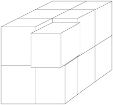
Figure 1.1: Sample decomposition of a 3-D mesh. The upper right corner box has been pulled out to show that the mesh has been subdivided along the x, y, and z axes.

For this simple problem, using the communication model above, we can estimate the time for a single step, using p nodes, as

(1.2)?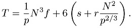

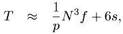
The first term is the floating-point work, which decreases proportionally with an increase in the number of processors p. The second term gives the cost of communicating each of the six faces to the neighboring processors, and includes both a term independent of the number of processors, and a term that scales as p^2/3, which comes from dividing the original domain into p cubes, each with N/p^1/3 along a side. Note that even for an infinite number of nodes, the time for a step is at least 6s (the minimum time or latency to communicate with each of the six neighbors). Thus it makes no sense to use an unlimited number of processors. The actual choice depends on the goal of the cluster:

• Minimize cost: In this case, you should choose nodes so that each subdomain fits on a node. In our example, if each node had 2 GBytes of memory, we would need at least 32 nodes (probably more, to leave room for the operating system and other parts of the application).

• Achieve a real-time constraint such as steps per second: In this case, T is specified and Equation 1.2 is solved for p, the number of nodes. Beware of setting T very small; as a rule of thumb, the floating-point work (the N³ f/p term) should be large compared to the communication terms. In this case, as p becomes large, and since

  

  in order to make the communication a smaller part of the overall time than that computation, we must have

  

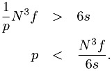
  For the typical values of s/f and for N = 1024, this bound is not very strong and limits p to a only few thousand nodes. For smaller N, however, this limit can be severe. For example, if N = 128 instead and if fast Ethernet is used for the network, this formula implies that p < 10.

Some notes on this example:

• We chose a three-dimensional calculation. Many two-dimensional calculations are best carried out on a single processor (consider this an exercise for the reader!).

• The total memory space exceeds that addressable by a 32-bit processor. But because we are using a cluster, we can still use 32-bit processors, as long as we use enough of them.

• The expected performance is likely to be a small fraction of the "peak" performance. We don't care; the cost of the cluster is low.

• If there are enough nodes, the problem may fit within the much faster cache memory (though this would require thousands of nodes for this example). In that case, the computing rate can be as much as an order of magnitude higher—even before factoring in the benefits of parallelism! This is an example of superlinear speedup: speedup that is greater than p on p processors. This is a result of the nonlinear behavior of performance on memory size and is not paradoxical.

• Latency here has played a key role in determining performance. In other computations, however, including ones for PDEs that use different decompositions, the bandwidth term may be the dominant communication term.

• Since each time step generates 64 GBytes of data, a high-performance I/O system is required to keep the I/O times from dominating everything else. Fortunately, Beowulf clusters can provide high I/O performance through the use of parallel file systems, such as PVFS, discussed in Chapter 19.