8.2 Choosing the Driving Table
The most important choice you make when putting together an execution plan is your choice of the driving table. You will rarely find a good execution plan without driving from the single best choice, and the best choice of driving table usually ensures at worst a pretty good plan, even if you pick the remainder of the join order quite haphazardly. I've stated that the rule for choosing the best driving table is simple: just drive from the table with the lowest filter ratio. Here, I make the case that such a simple rule almost always works and is really the only possible rule that is both simple and usually right.
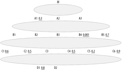
The dilemma for all optimizers, human or otherwise, is how to choose the best driving table without iterating through every join order or even a significant fraction of the join orders. Any fast method for choosing the driving table must depend on localized informationinformation that does not reflect the entire complexity of the query. To demonstrate the reasoning behind the simple rule to drive from the table with the lowest filter ratio, I discuss a problem with deliberately hidden details, hiding the full complexity of the query. Consider the partially obscured query diagram of Figure 8-2.
Figure 8-2. A partially hidden query diagram

What does such a diagram convey, even in the absence of the join links? Without the join links or join ratios, you can still say, with fair confidence:
M is the root detail table, likely the largest and least-well-cached table in the query. Call the rowcount of this table C.
A1, A2, and A3 are master tables that join directly to M.
All the other tables are also master tables and appear to be joined indirectly to M, through intermediate joins.
Even with this sparse information, you can deduce a key property of the cost of reading that largest and least-well-cached root detail table M:
The number of rows read from the root detail table will be no more than that table's rowcount (C) times the driving table's filter ratio.
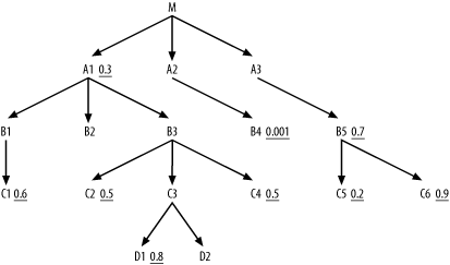
For example, even if table B4 holds the only filter you can reach before you join to M, driving from B4 with nested loops ensures that you read just one-thousandth of the rows in M. Figure 8-3 illustrates this case.
Figure 8-3. The query diagram with possible join links uncovered

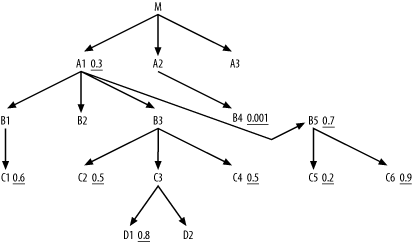
Of course, if B4 connects directly to more nodes with filters before it must join to M, you can do even better. However, as long as you choose nested-loops joins, you know immediately that the upper bound of the cost of the read of the root detail table is C x Fd, where Fd is the filter ratio for the chosen driving table. This explains the driving-table rule, which chooses the node with the lowest filter factor as the driving table. To drive home this point, Figure 8-4 rearranges the links in Figure 8-3 to make a new diagram that maximizes the advantage of an alternative to driving from B4.
Figure 8-4. The query diagram modified to minimize the disadvantage of driving from table A1

Now, if you drive from A1 or any node connected below it, you can pick up every filter except the filter on B4 before reaching M. The result is that you reach a number of rows in M equal to C x 0.0045 (C x 0.3 x 0.7 x 0.6 x 0.5 x 0.5 x 0.2 x 0.9 x 0.8), which is over four times worse than the cost of driving from B4. Furthermore, with a poor initial driving filter, the other early-table access costs will also likely be high, unless all those tables turn out to be small.
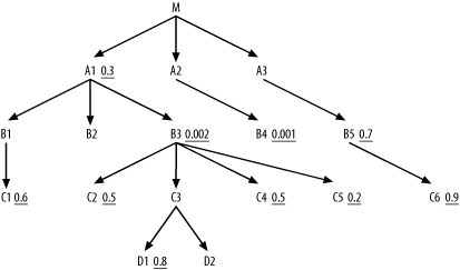
You might wonder whether this example is contrived to make the best driving filter look especially good, but the contrary is true: most real queries favor driving from the lowest filter ratio even more dramatically! Most queries have far fewer filters to combine, and those filters are more spread out across different branches under the root detail table than they are in this example. If you had two almost equally good filters, you could build a plausible-looking case for driving from the second-best filter if it had more near-neighbor nodes with helpful filters as well, such as in Figure 8-5.
Figure 8-5. A query diagram with competitive driving nodes

In this contrived case, B3 would likely make a better driving node than B4, since B3 receives so much help from its neighboring nodes before you would join to M. This might sound like a plausible case, and I don't doubt it can occur, but empirically it is rare. I haven't seen a case such as this in 10 years of tuning, mainly because it is so rare to find two very selective filters with roughly the same magnitude of selectivity in the same query. It is much more common that most of the selectivity of a query comes from a single highly selective condition.


