Star Optimization Evolution

There are several ways to optimize a query against a star schema design. But, the results are radically different in terms of runtime performance. Let's examine the evolution of these star schema query optimization techniques, their basic explain plan formats, and their performance results. We'll use the same example query from Chapter 4: How much beer and coffee did we sell in our Dallas stores during December 1998? The SQL code is as follows:

SELECT prod.category_name,
       sum (fact.sales_unit) Units,
       sum (fact.sales_retail) Retail
FROM   pos_day              fact,
       period               per,
       location             loc,
       product              prod
WHERE  fact.period_id     = per.period_id
  AND  fact.location_id   = loc.location_id
  AND  fact.product_id    = prod.product_id
  AND  per.levelx         = 'DAY'
  AND  per.period_month   = 12
  AND  per.period_year    = 1998
  AND  loc.levelx         = 'STORE'
  AND  loc.city           = 'DALLAS'
  AND  loc.state          = 'TX'
  AND  prod.levelx        = 'ITEM'
  AND  prod.category_name in ('BEER','COFFEE')
GROUP BY prod.category_name;

First-Generation

First-generation star schema query optimization consists of first joining a fact table to a dimension table and then iteratively joining the intermediate results table to each remaining dimension table. That translates into nested loops, and most DBAs already know that nested loops generally mean slow performance. Oracle 6 offered only first-generation star schema query optimization.

An explain plan for first-generation star schema optimization would look like Figure 5-1.

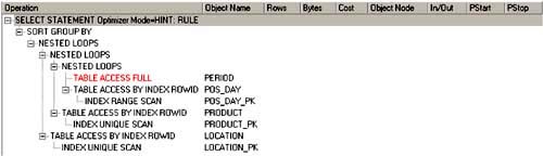
Example runtime statistics for a fact table with 7 million rows were found to be:

• 6,550 physical reads

• 698,742 logical reads

• 273 CPUs used by session

• 17.125 seconds elapsed time

There is absolutely no value in using this method for data warehousing. I merely disclose this information so that you understand the complete history of star schema tuning.

Second-Generation

Second-generation star schema query optimization consists of first Cartesian joining all dimension tables into one intermediate results table, and then joining that table to the fact table. This was Oracle 7's STAR hint. Just the fact that it does repetitive Cartesian joins should be enough to eliminate this choice for most people. Remember that Cartesian joining means combining every row of one table with every row from another table. That means a Cartesian join is a multi-table SELECT without a WHERE clause condition connecting those tables. Cartesian joining always means slow performance and should be avoided.

An explain plan for second-generation star schema optimization would look like Figure 5-2.

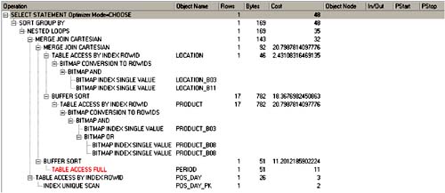
Example runtime statistics for a fact table with 7 million rows were found to be:

• 2,923 physical reads

• 156,154,547 logical reads

• 29,414 CPUs used by session

• 296.782 seconds elapsed time

Yes, that's over 156 million logical reads, with over 107 times as much CPU time and over 17 times as long to run! There is absolutely no case under which I can recommend using the STAR hint. It stinks. Don't use it.

Third-Generation

Third-generation star schema query optimization consists of Oracle's new, patented star transformation optimization technique, introduced in Oracle 8.0 and perfected by Oracle 9i. This method of accessing a fact table leverages the strengths of Oracle's bitmap indexes, bitmap operations, and hash joins. However, you must closely follow the advice of all subsequent sections regarding both initialization parameters and indexes to obtain such explain plans. In short and at a minimum, you must create a bitmap index on each fact table's dimension table's foreign key columns. In our example, that would mean:

• CREATE BITMAP INDEX POS_DAY_B1 ON POS_DAY (PERIOD_ID)

• CREATE BITMAP INDEX POS_DAY_B2 ON POS_DAY (LOCATION_ID)

• CREATE BITMAP INDEX POS_DAY_B3 ON POS_DAY (PRODUCT_ID)

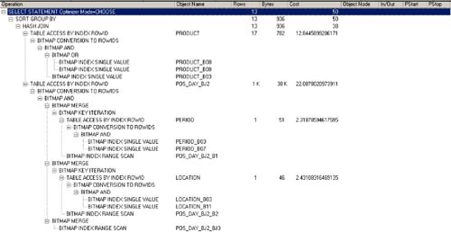
The entire index design will be discussed in more detail later. When done correctly, the explain plan for third-generation star schema optimization should look like Figure 5-3.

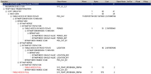
Example runtime statistics for a fact table with 7 million rows were found to be:

• 3,410 physical reads

• 22,655 logical reads

• 33 CPUs used by session

• 0.641 seconds elapsed time

How does it achieve such stellar results (no pun intended)? Oracle essentially rewrites the query as a non-correlated sub-query (shown below) and performs the explain plan in two distinct steps. First, it uses bitmap indexes on both the dimension and fact tables to greatly reduce the number of fact rows to return. Second, it joins the resulting limited set of fact rows to the dimension tables. This is a highly efficient and desirable explain plan to execute.

SELECT ...
FROM   pos_day              fact
WHERE  fact.period_id     in (
        SELECT period_id
        FROM   period
        WHERE  levelx       = 'DAY'
        AND    period_month = 12
        AND    period_year  = 1998 )
  AND  fact.location_id   in (
        SELECT location_id
        FROM   location
        WHERE  levelx = 'STORE'
        AND    city   = 'DALLAS'
        AND    state  = 'TX' )
  AND  fact.product_id    in (
        SELECT product_id
        FROM   product
        WHERE  levelx        = 'ITEM'
        AND    category_name in ('BEER','COFFEE') )
...;

Look again at Figure 5-3. While this particular plan shows a temporary table being used in the star transformation process, this is not always the case. The general format of a star transformation is:

• Hash join

  • Table access by index ROWID for fact

    • Bitmap AND

      • Bitmap MERGE

        • Table access by index ROWID for Dimension #1

          • Bitmap "AND"

            • Bitmap index scan

            • Bitmap index scan

            • … Repeats …

  • Bitmap index range scan for fact

• Bitmap MERGE

  • Table access by index ROWID for Dimension #2

    • Bitmap "AND"

      • Bitmap index scan

      • Bitmap index scan

      • … Repeats …

  • Bitmap index range scan for fact

• … Repeats …

As you'll see in the following section on index design, this optimization technique relies extensively on bitmap indexes for both dimension and fact tables. Look again at the explain plan: Only simple bitmap index scans appear?no b-tree index scans. If you get a plan with b-trees, you have not obtained a star transformation and the runtime will be substantially longer. Bitmap indexes are our best friends in data warehousing.

Fourth-Generation

Fourth-generation star schema query optimization consists of Oracle's new bitmap join indexes, introduced in Oracle 9i. Bitmap join indexes create a bitmap index on one table based on the columns of another table or tables. The idea is that bitmap join indexes hold pre-computed join results in a very efficient index structure. In theory, this should be the best possible route to go. The problem is that when people attempt to use this type of index, it can yield varying results, some of which are quite undesirable.

The first and most natural attempt at using bitmap join indexes is to replace existing third-generation solution bitmap indexes on the fact table's dimension table's foreign key columns. For example, instead of creating a bitmap index on each of our fact table's dimension table's foreign key columns, we would instead create bitmap join indexes. In DDL terms for our example, we would replace:

CREATE BITMAP INDEX POS_DAY_B1 ON POS_DAY (PERIOD_ID)

with:

CREATE BITMAP INDEX POS_DAY_BJ1 ON POS_DAY (PER.PERIOD_ID)
FROM POS_DAY POS, PERIOD PER
WHERE POS.PERIOD_ID = PER.PERIOD_ID

An explain plan for fourth-generation star schema optimization would look like Figure 5-4.

Example runtime statistics for a fact table with 7 million rows were found to be:

• 56,624 physical reads

• 60,714 logical reads

• 470 CPUs used by session

• 12.14 seconds elapsed time

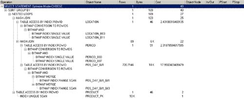
Wait just a minute. What happened? This was supposed to make things better, not worse. Look again at Figure 5-4. Although Oracle 9i's optimizer utilized the new bitmap join indexes, it also reverted back to using nested loops and b-tree indexes. And for most data warehouses, we never want to see b-tree indexes in our query explain plans?they'll run orders of magnitude slower than if using exclusively bitmaps. And for Oracle 8i, the explain plan would not have used any of the new bitmap join indexes. It would instead do a full table scan of our fact table! Lesson learned: A successful fourth-generation solution must be built on a third-generation foundation, not instead of. In other words, we need both bitmap indexes from above. We should let the Oracle query optimizer decide what's best. When done correctly, the explain plan should look like Figure 5-5.

Example runtime statistics for a fact table with 7 million rows were found to be:

• 5,833 physical reads

• 7,111 logical reads

• 79 CPUs used by session

• 3.640 seconds elapsed time

Look again at Figure 5-5. We essentially have the star transformation plan from Figure 5-3 with some very subtle changes. First, the temporary table transformation step is removed near the top of the plan (it's only necessary when temporary tables are being used during the star transformation process). And second, the table access full of the temporary table is replaced near the bottom of the plan with a bitmap range scan of the bitmap join index. But note that it follows our general star transformation pattern and yields a bitmap result to include in the bitmap merge process. So, we have a legitimate star transformation here with simply the addition of a bitmap join index.

Evolutionary Summary

Summarizing our results in Table 5-1, we see that the best overall results are achieved by the third-generation solution: the star transformation. It yields the best mix of physical versus logical I/O, with the lowest CPU usage and elapsed runtime. In other words, the star transformation is our target.