Case Studies

4.3.1 Convolutional Coder

As seen in the previous sections, the channel coding schemes CS-1, CS-2, and CS-3 are based on a convolutional code, a frequently used mechanism to improve the performance in a digital radio communication system. This code is used to introduce some redundancy in the data bit sequence, to allow the correction (at the receiver end) of errors that may occur on these data bits during transmission, due to propagation conditions, interference, RF impairments, and so on.

A convolutional code is a type of error correction code in which each k-bit information symbol to be encoded is transformed into an n-bit symbol. In many cases, k is equal to 1, which means that each bit of the sequence to be encoded is input one by one in the coder, and each input bit produces a word (also called a symbol) of n bits.

In such a code, the n output bits are not only computed with the k bits at the input, as in a block code, but also with the L - 1 previous input bits. The transformation is a function of the last L information symbols, where L is the constraint length of the code. This is the difference with block codes, for which only the input data bits are taken into account to compute the output bit sequence.

The ratio k/n is called the code rate. The degree of protection achieved by a code is increased when the code rate is decreased, which means that higher redundancy is introduced. A code is often characterized by as (n,k,L), where L is the constraint length of the code. This constraint length represents the number of bits in the encoder memory that affect the generation of output bits. A convolutional code can be implemented as a k-input, n-output linear sequential circuit with input memory m, as shown in Figure 4.13.

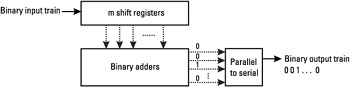Figure 4.13: Circuit for a convolutional code.

The coder structure may be derived in a very simple way from its parameters. It comprises m boxes representing the m memory registers, and n modulo-2 adders for the n output bits. The memory registers are connected to the adders.

The rule defining which bits are added to produce the output bits is given by the so-called generator polynomials. For example, for a ratio 1/2 code, 2 polynomials are used, as shown for the code defined by G0 and G1 on Figure 4.14, with

G0 = 1 + D³+D⁴

G1 = 1 + D +D³ + D⁴

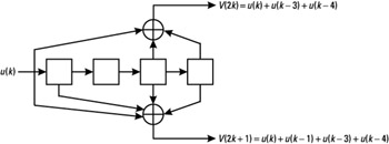
Figure 4.14: Circuit for the rate 1/2 code defined by G0 and G1.

In this notation, D represents the delayed input bit. If we denote by u(n) and v(n) respectively the input and output sequences of the coder, we have

(4.6)

(4.7)

Usually, we have u(k) = 0 for k < 0. This code defined by GO and G1 generates two output bits for every 1 input bit. Its constraint length L is equal to m + 1, which is 5 in this case.

For this example, suppose that the initial state of the registers is all zeros (0000), and that the sequence 1001 is presented at the input. The following operations are performed (see Figure 4.15):

• The first input bit "1" generates the two bits "11" on the output (1 + 0 + 0 = 1 and 1 + 0 + 0 + 0 = 1), and the state of the registers becomes 1000, since the input bit one moves forward in the registers.

• The input is now the bit "0," which generates the pair of bits "01," and the new state is 0100.

• The next input is "0:" it generates the pair "00," with a shift in the registers to the state 0010.

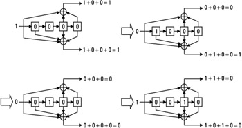
Figure 4.15: Example with the input bit sequence 1 0 0 1.

A "1" is entered in the coder, so the output becomes "00."

In this example, the complete output sequence is therefore 11010000.

At the end of the coding process, for each coded block, a fixed sequence of bits is usually placed at the input of the coder, in order to bring the coder to a known state. This will be described further in the next section, since it is useful to the decoder. This fixed sequence is called the tail bit.

The codes used in GPRS are defined by the polynomials GO and G1, presented above, that are also used for several other GSM logical channels (including TCH/FS and SACCH). It is interesting to notice that the coding schemes CS-1 to CS-3 are all based on the same generator polynomials, although not resulting in the same code. This is due to the fact that the puncturing technique is used to change the code rates. With the coder structure presented above, the achievable code rates are 1/2, 1/3, 1/4, 2/3, 2/5, and so on, since k and n are integer values. These codes are often denoted as "mother codes." Puncturing is a method that allows the code rates to be changed in a very flexible manner. This is done in the transmitter by suppressing some of the bits of the coder output sequence, in particular positions. These positions are known to the receiver, which can replace the erased bits with zeros. The decoding process is then just the same as for the basic mother code. Many higher rated codes can therefore be formed, which allows for the provision of different degrees of protection, and adaptation of the bit rate to the available bandwidth.

Taking into consideration the CS-3 case, 338 bits are input to the 1/2 coder, resulting in 676 coded bits, and 220 of these bits are punctured, so that 456 bits are actually transmitted in a radio block. The overall rate of the code is in this case 338/(676 - 220) ≈ 0.741. The 220 punctured bits are such that among the 676 coded bits, the bit positions 3 + 6j and 5 + 6j, for j = 2, 3, ..., 111 are not transmitted. Table 4.15 shows the code rates of the CS-1 to CS-3 codes.

4.3.2 Viterbi Decoding

There are several different approaches with respect to the decoding of convolutional codes. The Viterbi algorithm is most often used. This algorithm, introduced by Viterbi [2] in 1967, is based on the maximum likelihood principle. This principle relies on intuitive behavior in comparing the received sequence to all the binary sequences that may have been coded, and choosing the closest one. Once the coded sequence closest to the receive sequence is identified, the input bits of the code can be deduced. Of course, the complexity of such an exhaustive comparison is not reasonable if we consider the implementation point of view, and it is the purpose of the Viterbi algorithm to reduce the number of comparisons, as will be explained later in this section.

First of all, it is convenient to introduce the maximum-likelihood concept. Let us assume that the sequence of information bits u = (u₀, ... , u_N-1) is encoded into a code word v = (v₀, ... , v_M-1), and that the sequence r = (r₀, ... , r_M-1) is received, on a discrete memoryless channel (DMC). This very simple channel is shown in Figure 4.16: The transmitted bits can either be transmitted correctly, with the probability 1 -p, or with an error, with the probability p. This channel has no memory in the sense that consecutive received bits are independent.

Figure 4.16: Discrete memoryless channel.

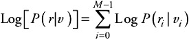
The decoder can evaluate the maximum-likelihood sequence as the codeword v maximizing the probability P(r|v). On a memoryless channel, this probability is

where P(r_i|v_i) is the channel transition probability of the bit i, since the received symbols are independent from each other.

We can therefore derive that

Indeed, if we suppose that P(r_i|v_i) = p if r_i ≠ v_i, and P(r_i| v_i) = 1 -p if r_i = v_i, then we have

(4.8)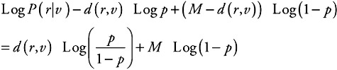

where d(r, v) is the Hamming distance between the two words r and v; that is, the number of positions in which r and v differ. For instance, the distance d(100101,110001) is 2.

What is important to understand from (4.8) is that, on a DMC, maximizing the likelihood probability P(r|v) is equivalent to minimizing the Hamming distance between the received word r and the possible transmitted coded sequence v. Indeed, the maximal value for a probability is 1, so Log P(r|v) maximal value is 0. THis characteristic is used for the decoder, as described in this section.

The decoding relies on a representation of the code called a trellis. A trellis is a structure that contains nodes, or states, and transitions between these states. The states represent the different combinations of bits in the registers. There are 2^L-1 such combinations, L being the constraint length of the code.

For instance, for the code presented in Figure 4.17, based on the polynomials g₁ (D) = 1 + D + D² and g₂(D) = 1 + D², there are four states: 00, 01, 10, and 11. The four possible states of the encoder are represented as four rows of dots. There is one column of four dots for the initial state of the encoder, and it is repeated for each step of the algorithm.

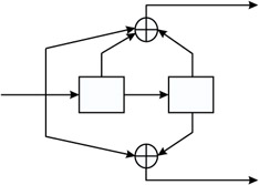
Figure 4.17: Example of 1/2 convolutional code.

The coder in a given state changes to another state according to the input bit. A dashed arrow represents a 0 input bit, and a full line represents a 1 at the input of the encoder. For instance, if the coder is in the state 01, it will either change to the state 00, if the input bit is equal to 0, or 10, if the input bit is equal to 1. This is represented by the transitions, or arrows, in the trellis diagram.

For a 5-bit message at the input of the coder, for instance, there will be five steps in the algorithm. The labels on the transitions are the outputs of the coder. With the 1/2 code of our simple example, the transition between the states 01 and 00 is labeled 11. Indeed, if the state is 01, and the bit 0 is input to the coder, the output bits are 0 + 0 + 1 = 1, and 0 + 1 = 1 (remember that all the operations are performed modulo 2).

A trellis for this code is also shown in Figure 4.18. Note that once the transitions between the pair of states are made, this basic set of transitions can be repeated N times, N corresponding to the size of the input bits block. As we will see, each of these N repetitions of the trellis basic structure will correspond to a step in the algorithm.

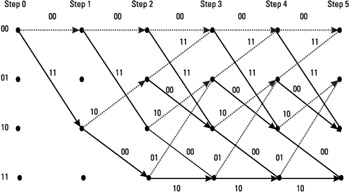
Figure 4.18: Associated trellis diagram for the example code.

A transition in the trellis is also denoted as a branch, and a series of several branches, between one state and another, is called a path in the trellis.

Also notice that the initial state of the encoder is 00, so the arrows start out at this state. No transitions from the other states are represented at the beginning of the trellis. After two steps, all the states are visited, since all the combinations of bits are possible in the registers. The structure of the trellis diagram helps to compute the maximum-likelihood sequence. The principle of the Viterbi algorithm is to select the best path according to the metric given by the Hamming distance.

For the sake of example, let us suppose that the coded sequence 00 11 10 00 10 is transmitted, and that the receiver receives the sequence 00 11 10 01 10. Let us run the algorithm on this sequence to show how it can determine what the correct sequence is.

For each received pair of channel symbols, a metric is computed, to measure the Hamming distance between the received sequence and all of the possible channel symbol pairs. From step 0 to step 1, there are only two possible channel symbol pairs that could have been received: 00 and 11. The Hamming distance between the received pair and these two symbol pairs is called a branch metric.

The two first received bits are 00, so between step 0 and step 1, the branch metrics are calculated as follows:

• The transition between states 00 and 00 is marked with the label 00, so the branch metric is d(00,00) = 0.

The transition between states 00 and 10 is labeled 11, so the branch metric is d(00,11) = 2.

This process is then repeated for the transition between steps 1 and 2. The received sequence is then 11, and there are four transitions to explore:

• Between states 00 and 00 the branch metric is d(11,00) = 2.

• Between states 00 and 10 the branch metric is d(11,11) = 0.

• Between states 10 and 01 the branch metric is d(11,10) = 1.

• Between states 10 and 11 the branch metric is d(11,00) = 2.

The algorithm really starts after step 2, since there are now two paths that converge, for each state of the trellis.

We have seen that for each pair of received bits, the branch metrics associated with the transitions between states are calculated. In the algorithm, a path metric is also computed, as the sum of the branch metrics that compose the path. These cumulated metrics are calculated for each path that converges to a given node. Once these cumulated metrics are computed, the algorithm selects for each node the so-called survivor. A survivor is the path whose cumulated metric is the smallest, between the paths that merge to a given state.

In our example, the survivor, at step 3, for the state 01 is the path that comes from the state 10. The path that comes from the state 11 is removed. Table 4.16 gives, for each step, the estimation of the survivor path metric at each node of the trellis.

The idea is that each path in the trellis from state 00, at step 0, to one of the four states 00, 01, 10, and 11, at step n, represents a different sequence that may have been received. Indeed, there are 2ⁿ paths of length n between state 0 and the four states at step n. The sequences represented to one path is the series of labels on each of its transitions.

What is important to understand is that for each state, one of the two paths that converge to this state is better than the other, with respect to the Hamming distance. When the minimum value between the two path metrics is chosen, this means that the path corresponding to this metric is selected, the other being removed. Instead of estimating the Hamming distance between all the possible sequences of n bits and the received sequence, the algorithm deletes half of the possible combinations at each step. It is indeed shown that for a given node, if the path P1 has a higher cumulated metric than the survivor P2, it will never be the maximum likelihood sequence. This is clear since for the next steps, P2 will always be better than P1 with regard to the path metric.

In our example, at step 5, the survivors corresponding to each step are depicted in Figure 4.19.

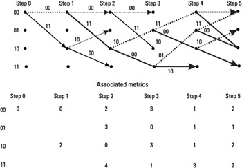
Figure 4.19: Representation of the survivors at step 5.

This process of choosing the survivor for all the states is repeated until the end of a received sequence. Once this is reached, the trace-back procedure is performed. This procedure corresponds to:

• The selection of the best survivor. This is either the path that has the smallest metric among all four survivors, at the last step, or the survivor that corresponds to the known ending state. Indeed, if tail bits are used at the encoding, to bring the coder to a known state, the decoder does know which survivor to select. For instance, in our example, two bits equal to 0 will bring the coder to the state 00. If the receiving end knows that the state 00 is reached at the end of the sequence, it is able to perform the decoding more effectively (it will not chose the survivor from another state and thus will avoid errors in the end of the sequence).

• The determination of the maximum likelihood transmitted sequence. This is done by examining each branch of the trellis, to see if it corresponds to a 0 input (dashed line), or a 1 input (full line). The series of 0 and 1 represented by the arrows of the path give the decoded sequence.

In our example, if we suppose that step 5 is the last step, we see that the best survivor is the one from state 01, since its Hamming distance is 1. This means that the received bit sequence differs from one bit to the sequence corresponding to this path (i.e., the sequence of the labels on each branch of this path). In this case, the transmitted sequence corresponding to the received bits 00 11 10 01 10 would be 01010. We also see that this input sequence produces the bits 00 11 10 00 10 in the encoder, which means that an error has occurred at the position 8 in the sequence, but the sequence was correctly decoded anyhow.

Of course, this is just an example, and the block size is usually longer than that, before the trace-back is performed (in the CS-3 case, for instance, 338 steps of the algorithm are executed, on a 16-state trellis). Note that the efficiency of the decoding process is increased if the number of steps is high.

The decoding method that we have seen in this example can be used in a similar way for any k/n code, and can be summarized as follows:

• Notations

  • N is the length of the data information sequence;

  • L is the constraint length of the code.

• For each step from t = 0 to N - 1

  • For each state from s = 0 to s = 2^L-1

    Estimation of the 2^k branch metrics that converge to the state s (Hamming distance between the received sequence and the sequence corresponding to the transition);

    Estimation of the path metrics for all the paths that converge to s;

    Determination of the survivor for state s: it is the path that has the minimum path metric, among all the paths that converge to s.

• Selection of either the best survivor among the 2^L-1 states at stage N- 1 (the one that has the minimum path metric), or the survivor corresponding to the known ending state (if tail bits are used).

• Trace back to determine the input bit sequence corresponding to this best survivor.

The major interest of this algorithm is that its complexity is proportional to the number of states (number of operations proportional to N × 2^L-1). This is a great complexity improvement compared with the 2^N comparisons that would be needed to explore all the possible received sequences.

The algorithm was described in this section for the DMC, that is, by supposing that the decoder input is a binary sequence, via hard decisions on the received samples. Convolutional codes are often based on soft decoding, which means that the input of the decoder is a sequence of "analog" samples, or soft decisions.

Examples of soft decisions would be:

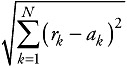
• Binary samples ±1 on an additive white Gaussian channel. The received samples r_k are Gaussian and uncorrelated. In this case, it can be shown that the metric to be used to compute the maximum likelihood of a path in the trellis diagram is the Euclidean distance. If a sequence r_k is received, the Euclidean distance between this sequence and a sequence of N binary symbols a_k in {±1}^N would be

  

• Equalizer soft decisions. In radio communication systems, the outputs of the equalizer are usually soft decisions on the received bits. This means that instead of delivering ±1 values, the equalizer output is a sequence y_k = b_kP_k, where b_k is a binary symbol ∊ {±1}, and p_k is proportional to the probability associated with this symbol. The idea is that the equalizer provides for each received bit, an estimation of the probability that this bit is the original bit that has been sent. A soft decision is therefore a reliability value, which may be used to increase the decoding capability. In such a case, the metric used in the Viterbi algorithm can be.

  

If y_k and a_k have the same sign, the metric is increased; otherwise, it is decreased. In this case, the Viterbi algorithm is used to select the path that maximizes this metric.

4.3.3 MS Measurements

This section describes the estimation principles for the measurements that are reported by the MS to the network.

RXLEV

As seen in the previous sections, this parameter corresponds to a received signal strength measurement on:

• The traffic channels if the MS is involved in a circuit-switched communication (GSM speech or data), or in GPRS packet transfer mode;

• On the BCCH carriers of the surrounding cells, for circuit- and packet-switched modes;

• On carriers indicated for interference measurements, in packet transfer or packet idle modes (these measurements are mapped on the RXLEV scale).

This received signal strength is evaluated on the baseband received I and Q signals, usually after the analog-to-digital conversion. The estimation of the power in dBm is done on samples, (I_k) and (Q_k), quantified on a certain number of bits:

(4.9)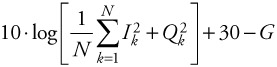

where N is the number of samples used for the estimation, and G is the gain of the RF receiver in decibels, including the analog-to-digital converter gain. To get the result in dBm, the power estimation is converted to decibels (P_dB = 10 · log(P_Watt)), and the term 30 is added (P_dBm = 10 · log(P_mWatt) = P_dB + 30). Note that the receiver gain must be deducted from the result to estimate the received power level at the antenna.

Several estimations in dBm, taken from different time slots, are averaged for the computation of the RXLEV. Usually, each estimation is estimated on one received burst, or less than one burst in the case of the surrounding cells monitoring. Indeed, it may happen for some multislot cases that the MS must reduce its measurement window, in order to increase the time left for channel frequency switching. The precision will of course depend on the number of samples N used for each estimation, and on the number of estimations that are averaged.

The measured signal level is then mapped onto a scale between 0 and 63, and reported to the network.

RXQUAL

As seen in Section 3.3.1.5, this parameter is an estimation of the BER on the downlink blocks at the demodulator output (no channel coding). This estimation is obtained by averaging the BER on the blocks intended for the MS that are successfully decoded, in the sense that no error is detected by the CRC check. On these correctly decoded blocks, it is assumed that the convolutional code, for CS-1 to CS-3, is able to correct all the errors that have occurred on the physical link. This is a reasonable assumption since the probability that an error on the decoded bit remains undetected by the CRC decoder is very low.

Since we assume that the errors are all corrected by the convolutional code, a simple way of estimating the BER on the demodulated bits of one block is to proceed as follows:

• Once a block, mapped on four bursts on a given PDCH, is received, the soft bit decisions delivered by the equalizer are used for the convolutional decoding.

• The CRC of the decoded block is checked, and if no error is detected, the block is used in the BER estimation process, if it is addressed to the mobile; otherwise, it is skipped.

• If the decoded block is kept, it is reencoded by the convolutional encoder, to produce the coded bits, just as in the transmitter.

• These coded bits are compared with the hard decisions that are delivered by the equalizer. The number of detected errors is simply divided by the length of the coded block-that is, 456 bits-to produce an estimate of the BER.

The estimated BER on several blocks is then averaged to compute the RXQUAL, which is a value between 0 and 7. This method is summarized in Figure 4.20. Note that this estimation is not possible on the blocks that are not correctly decoded (CRC check), since it cannot be assumed on these blocks that the convolutional decoder has corrected all the errors (otherwise the CRC check would be okay), and therefore the accuracy cannot be met.

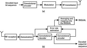
Figure 4.20: BER estimation for the RXQUAL measurement- operations in the (a) transmitter and (b) receiver.

This method cannot be used if the code is CS-4, since CS-4 has no convolutional coding. For this reason, reporting of a precise estimate of the BER is not requested in CS-4, and the MS is allowed to report RXQUAL = 7 (this corresponds to a BER greater than 12.8%).

4.3.4 RF Receiver Structures

This section is a summary of the architectures commonly in use in the MS and BTS receivers. Of course, the implementation of the receiver is not described in the standard, but it will be designed by the manufacturers to meet the specified performance. This case study presents the basics of RF receiver architectures, in order to show the different constraints of the recommendations and their impact on the practical implementation. It is suggested that the reader first review Section 4.2 covering the GPRS RF requirements. For a detailed presentation of the RF architecture and implementation issues, refer to [3].

4.3.4.1 Intermediate Frequency Receiver

The purpose of the RF receiver is obviously to receive the RF modulated signal, and to transpose this signal to the baseband I and Q signals. These signals are then digitized (in the ADCs), and treated by a set of demodulation algorithms (CIR estimation, time and frequency synchronization, equalizer, decoding, and so on).

The intermediate frequency (IF) structure, or superheterodyne receiver, is shown in Figure 4.21. The receiver front-end contains a band selection filter (to select all the downlink bands of the system), and a low noise amplifier (LNA). Two stages are then used for the down-conversion of the RF signal to the baseband I and Q signals. The basic principle is the conversion of the RF carrier to a fixed IF by mixing it with a tunable LO. A bandpass filtering is then applied at this IF frequency, prior to a second conversion into baseband.

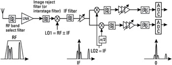
Figure 4.21: IF receiver architecture.

In the first stage, the mixing of the RF input signal to the RF ± IF LO has the effect of transposing the RF signal down to the IF. This is due to the fact that the LO signal, A₀ · cos(2πf_LOt), and the RF wanted signal A(t) · cos[2πf_RFt + φ(t)] are placed at the mixer's input. f_LO and f_RF are the LO and RF frequencies, A₀ is the amplitude of the LO sinusoidal signal, A(t) is the amplitude modulation (AM) (with the ideal GMSK signal, it is constant), and φ(t) is the phase modulation signal.

The result of this product is

(4.10)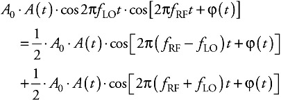

If, for instance, f_LO = f_RF -f_IF the result is

The band pass filtering of this signal removes the second term, and the result is a modulated signal transposed to an IF central frequency. By changing f_LO, all the RF channels can be converted to a constant IF. The second stage of this architecture is needed to make the downconversion from IF to baseband (around 0 Hz central frequency). In order to do so, each of the IF LO in-phase A₁ · cos(2πf_IFt) and quadrature

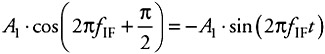
signals are mixed with the IF modulated signal.

This produces the two signals I(t)αA(t) · cosφ(t) and Q(t)αA(t) · cosφ(t). Note that with f_LO = f_RF + f_IF, the result is similar.

I(t) is called the in-phase signal, and Q(t) the quadrature signal. The complex signal I(t) + j · Q(t) is the baseband received signal, also called the complex envelope of the RF signal. Note that the RF signal can be written I(t) · cos(2πf_RFt) - Q(t) · sin(2πf_RFt).

One important issue with the IF receiver architecture is the problem of the image frequency. This problem is illustrated in Figure 4.22. In the first stage of the receiver, the RF signal is converted to IF, since, in our example, f_LO = f_RF -f_IF. In this case, the signal that is present around f_LO - f_IF, at the input of the receiver, is also downconverted to IF and added to the modulated signal. This signal may for instance be another carrier of the system, or an interference out of the reception band, depending on the choice of IF frequency. After downconversion to baseband, this unwanted signal is added to the modulated signal, resulting in a cochannel interference, thus degrading the performance of the receiver.

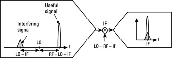
Figure 4.22: Problem of image frequency in IF architecture.

For this reason, the IF LO frequency is often chosen to be large enough so that the image frequency (f_LO -f_IF in our example) is filtered out by the RF reception band filter, placed at the receiver front end. Such filter allows the signal placed at the image frequency to be partially removed, resulting in an improved signal to interference ratio at baseband.

As shown in Figure 4.21, an image reject filter, also called interstage filter, may also be placed before the RF mixer stage, in order to filter out the signal present at the image frequency. Note that between the RF and IF mixing stages, an IF filter is usually used to perform the channel filtering. Such a filter is usually very selective, and allows the suppression of adjacent channel interference and wideband noise.

In the IF architecture, the current technology does not permit integration of the interstage and IF filters, which is the major drawback of this scheme. Indeed, it requires costly and bulky external filters.

4.3.4.2 Zero-IF Receiver

The second classic RF receiver scheme is the zero-IF structure, or direct conversion receiver, which is based on a single downconversion stage (see Figure 4.23). This means that there is only one LO, with f_LO = f_RF, so that the I and Q signals are delivered at the output of the RF mixers. Note that the receiver front-end is similar to the IF case.

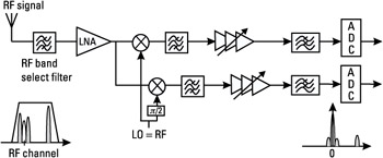
Figure 4.23: Zero-IF receiver architecture.

The benefit of having a single downconversion stage is of course a reduction in the components number, as compared with the IF scheme. Indeed, the interstage and IF filters are not required in this structure. For this reason, this architecture is one of the most cost-effective solutions, well suited for a mobile phone design, for which the cost and surface are critical issues. The drawback of this architecture is the so-called dc offset generated together with the baseband-modulated signal. The dc offset is a constant signal that is added to the signal of interest. This offset may be caused by several sources, as depicted in Figure 4.24.

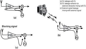
Figure 4.24: The dc offset sources in the ZIF receiver-

One source is the LO leakage due to the limited isolation between the LO and the input of the mixer and LNA [Figure 4.24(a)], which is mixed with the LO signal itself. The leakage may also reflect on external obstacles before this self-mixing effect occurs [Figure 4.24(b)]. Similarly, there may be some self mixing of a high-power interference signal (blocking), as shown in Figure 4.24(c), leaking from the LNA or mixer input to the LO. This means that a small portion of the interference power is coupled onto the LO. The mixing of this leakage signal with the interfering signal itself results in a dc component.

All these phenomena have the same effect: two signals at the same RF frequency are mixed together and produce a constant, or dc, on the baseband I and Q. In order to cope with the dc problem, analog solutions are possible, based on a dc compensation on the I and Q baseband signal. However, such solutions are not fully efficient in a context of varying radio conditions. Software solutions are therefore often required, to compensate for the residual dc on the digitized I and Q signals.

For Figure 4.24(c), one problem is that the blocking signal might not be synchronized with the receive burst. One can think of a carrier of the GSM system in the same band of operation, and therefore not filtered by the receive band filter. This carrier is not necessarily synchronized with the received channel frequency (different BTSs are not synchronized with one another): this raises the problem of a dc step occurring during the received burst (the beginning of the interfering carrier burst is not synchronized with the beginning of the desired carrier burst). The receiver has no information on the position and level of this step, and therefore complex digital processing techniques are needed to remove the step.

This problem arises in the conditions of the AM suppression characteristics (see Section 4.2.3.5). In this case, the RF mixers detect the envelope of the blocking signal and reproduce it on their output (see Figure 4.25), due to the RL-to-LO coupling and second-order nonlinearity distortion. Digital signal processing techniques may therefore be required to detect the step, to find out its position in the receive burst and its level. It is then possible to suppress this dc step. These problems concerning the dc offset may require the increase of the ADC's dynamic range, to avoid their saturation.

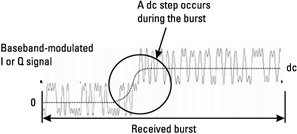
Figure 4.25: AM problem.

Another drawback of the zero-IF scheme compared to the IF solution is the possible degradation of the receiver noise figure (NF), which also means a degradation of the sensitivity level. This is due to the fact that the IF architecture performs better in terms of selectivity (filtering of the signal to remove the noise, interference, and blocking signals) in the IF stage. Therefore, the RF filtering prior to the LNA may be relaxed in the IF scheme compared to the zero-IF one. This distribution of the filtering allows the insertion loss of the receiver band filter to be reduced, leading to a better noise figure (see Section 4.3.5.1).

4.3.4.3 Near-Zero-IF Receiver

To avoid the problem of the dc offset, an interesting architecture is the low IF, or near-zero IF, which is actually a special case of the superheterodyne receiver (see Figure 4.26). In this scheme, the RF mixers' downconversion stage is used to translate the RF signal to IF, and the IF signal is directly digitized and converted afterward to baseband in the digital part of the system. The IF will therefore be sufficiently low to allow a practicable ADC implementation (the ADC sampling frequency will be at least two times greater than the maximum input signal frequency, to respect the Shannon theorem, but the oversampling ratio is at least four in practical cases). The dc offset can be removed at this stage, prior to the second downconversion to baseband, which is done in the digital part of the system.

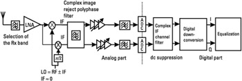
Figure 4.26: Near-zero-IF architecture.

The image frequency rejection is a real issue in this method, since the image frequency is within the receive band, so it is not filtered out by the front-end filter (Rx band selection filter). Therefore, if the image is not rejected, the interference caused on the baseband signal may be very high, often higher than the desired signal itself. For instance, in an implementation where the IF is equal to 100 kHz, the image frequency is 200 kHz away from the RF carrier that needs to be demodulated, so it is an adjacent channel interference. This interference is specified 9 dB higher than the signal of interest in the GSM adjacent channel requirement. It is therefore very important to remove the image in the mixers, or with a complex polyphase filter after the first downconversion to IF. This filter acts as an all-pass filter for the positive frequencies, and as a bandstop filter for the negative frequencies. The efficiency of this filter may be dependent upon the quadrature accuracy (only low phase and amplitude mismatches are tolerated). Note that a great part of the channel filtering is usually achieved in the digital part of the system, which requires an important ADC dynamic range (interfering signals are not completely removed prior to the ADC stage). A detailed description of this scheme is given in [4].

4.3.5 RF Receiver Constraints

4.3.5.1 NF

One of the most important specifications in a receiver is the sensitivity it is able to achieve, that is, the minimum level of signal power that can be received with an acceptable signal-to-noise ratio (SNR), ensuring a sufficient level of BER. The smaller the BTS and MS sensitivity levels, the better the performance of the whole system will be, since the link quality will be better in areas covered with large cells.

Factors influencing the sensitivity level are:

• The receiver NF, which is a measure of the SNR degradation at the output of the analog receiver, compared to the input;

• The channel filtering, which modifies the SNR, since it partly removes the noise;

• The performance of the baseband demodulation algorithms, which is characterized by BER curves (or BLER, see Section 4.2.3) versus SNR (the SNR is often under form of E_b/N₀, that is, the ratio of the signal energy during a bit period relative to the energy of the noise during this same period);

• RF imperfections;

• Imperfections in the digital signal processing part.

Knowing the capability of the demodulation algorithms to achieve the level of performance required in the recommendations (BER, BLER, and so on), in the presence of RF and digital signal processing impairments, the RF system designer can derive the NF needed in the receiver.

Below we analyze one by one the factors listed above.

Receiver NF

The NF is a measure of the SNR degradation as the signal passes through the system. It is determined by measuring the ratio of the SNR at the output to that at the input of the receiver.

(4.11)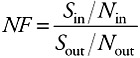

where:

• S_out and N_out are the wanted signal and noise powers at the output of the RF reception chain;

• S_in and N_in are the wanted signal and noise powers at the input of the RF reception chain.

The overall receiver NF may be calculated from the NFs of the different elements of the system, with the Friss equation:

(4.12)

In this equation, NF_i and G_i represent the NF and gain of stage i. The NF is usually expressed in decibels: NF_dB = 10 · log(NF).

What can be observed from (4.12) is that the higher the gain in the first stages, the lower the overall NF. Indeed, for the same total gain G₁ + G₂ + ... + G_N-1, the receiver NF will be lower if G₁ and G₂ are higher. A high gain in the receiver front end has the effect of "masking" the NF of the following stages. This is why, for instance, in the zero-IF architecture, the overall NF may not be as good as in the IF architecture: in the IF

Back Cover GPRS for Mobile Internet Chapter 1: Introduction to the GSM System General Concepts GSM Services Network Architecture Radio Interface References Chapter 2: GPRS Services GPRS MS Classes Client-Server Relation Quality of Service Third-Generation Partnership Project References Selected Bibliography Chapter 3: Overview of GPRS GPRS Logical Architecture Transmission and Signaling Planes Radio Interface BSS Architecture Mobility PDP Context BSS Packet Flow Context Definition Gb Interface GPRS Backbone Network Architecture Reference Selected Bibliography Chapter 4: Radio Interface: Physical Layer PLL RF Physical Layer Case Studies References Selected Bibliography Chapter 5: Radio Interface: RLC/MAC Layer RLC/MAC Block Structure Broadcast Information Management Cell Reselection Listening to MS Paging Blocks Radio Resource Allocation RLC TBF Release Case Studies Reference Selected Bibliography Chapter 6: Gb Interface Frame Relay Basics Addressing over Gb NS Layer BSSGP Layer Case Studies References Selected Bibliography Chapter 7: Signaling Plane GMM PDP Context Management GTP Layer for the Control Plane Reference Selected Bibliography Chapter 8: User Plane Packet Transmission Between MS and SGSN GTP Layer for the User Plane IP Packet Sending Within GPRS PLMN Interworking with External Networks Reference Selected Bibliography List of Acronyms List of Figures List of Tables