6.3 Simple Examples
Nothing illustrates the method better than examples, so I demonstrate the method using the query diagrams built in Chapter 5, beginning with the simplest case, the two-way join, shown again in Figure 6-1.
Figure 6-1. A simple two-way join
Applying Step 1 of the method, first ask which node offers the best (lowest) effective filter ratio. The answer is E, since E's filter ratio of 0.1 is less than D's ratio of 0.5. Driving from that node, apply Step 2 and find that the best (and only) downstream node is node D, so go to D next. You find no other tables, so that completes the join order. Following the rules for a robust execution plan, you would reach E with an index on its filter, on Exempt_Flag. Then, you would follow nested loops to the matching departments through the primary-key index on Department_ID for Departments. By brute force, in Chapter 5, I already showed the comforting result that this plan is in fact the best, at least in terms of minimizing the number of rows touched.
|
6.3.1 Join Order for an Eight-Way Join
So far, so good, but two-way joins are too easy to need an elaborate new method, so let's continue with the next example, the eight-way join. Eight tables can, in theory, be joined in 8-factorial join orders (40,320 possibilities), enough to call for a systematic method. Figure 6-2 repeats the earlier problem from Chapter 5.
Figure 6-2. A typical eight-way join
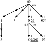
Following the heuristics outlined earlier, you can determine the optimal join order for the query diagrammed in Figure 6-2 as follows:
Find the table with the lowest filter ratio. In this case, it's C, with a ratio of 0.0002, so C becomes the driving table.
From C, it is not possible to drive down to any table through a primary-key index. You must therefore move upward in the diagram.
The only way up from C is to O, so O becomes the second table to be joined.
After reaching O, you find that you can now drive downward to OT. Always drive downward when possible, and go up only when you've exhausted all downward paths. OT becomes the third table to be joined.
There's nothing below OT, so return to O and move upward to OD, which becomes the fourth table to be joined.
The rest of the joins are downward and are all unfiltered, so join to S, P, and ODT in any order.
Join to A at any point after it becomes eligible, after the join to S places it within reach.
|
Therefore, you find the optimum join order to be C; O; OT; OD; S, P, and ODT in any order; and A at any point after S. This dictates 12 equally good join orders out of the original 40,320 possibilities. An exhaustive search of all possible join orders confirms that these 12 are equally good and are better than all other possible join orders, to minimize rows visited in robust execution plans.
This query diagram might strike you as too simple to represent a realistic problem, but I have found this is not at all the case. Most queries with even many joins have just one or two filters, and one of the filter ratios is usually obviously far better than any other.
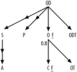
For the most part, simply driving to that best filter first, following downward joins before upward joins, and perhaps picking up one or two minor filters along the way, preferably sooner rather than later, is all it takes to find an excellent execution plan. That plan is almost certainly the best or so close to the best that the difference does not matter. This is where the simplified query diagrams come in. The fully simplified query diagram, shown in Figure 6-3, with the best filter indicated by the capital F and the other filter by lowercase f, leads to the same result with only qualitative filter information.
Figure 6-3. Fully simplified query diagram for the same eight-way join
I will return to this example later and show that you can slightly improve on this result by relaxing the requirement for a fully robust execution plan and using a hash join, but for now, I focus on teaching complete mastery of the skill of optimizing for the best robust plan. I already showed the 12 best join orders, and I need one of these for further illustration to complete the solution of the problem. I choose (C, O, OT, OD, ODT, P, S, A) as the join order to illustrate.
6.3.2 Completing the Solution for an Eight-Way Join
The rest of the solution is to apply the robust-plan rules to get the desired join order in a robust plan. A robust plan calls for nested loops through indexes, beginning with the filter index on the driving table and followed by indexes on the join keys. Here is the best plan in detail (refer back to Chapter 5 for the original query and filter conditions):
Drive to Customers on an index on (Last_Name, First_Name), with a query somehow modified to make that index accessible and fully useful.
Join, with nested loops, to Orders on an index on the foreign key Customer_ID.
Join, with nested loops, to Code_Translations (OT) on its primary-key index (Code_Type, Code).
Join, with nested loops, to Order_Details on an index on the foreign key Order_ID.
Join, with nested loops, to Code_Translations (ODT) on its primary-key index (Code_Type, Code).
Outer join, with nested loops, to Products on its primary-key index Product_ID.
Outer join, with nested loops, to Shipments on its primary-key index Shipment_ID.
Outer join, with nested loops, to Addresses on its primary-key index Address_ID.
Sort the final result as necessary.
Any execution plan that failed to follow this join order, failed to use nested loops, or failed to use precisely the indexes shown would not be the optimal robust plan chosen here. Getting the driving table and index right is the key problem 90% of the time, and this example is no exception. The first obstacle to getting the right plan is to somehow gain access to the correct driving filter index for Step 1. In Oracle, you might use a functional index on the uppercase values of the Last_Name and First_Name columns, to avoid the dilemma of driving to an index with a complex expression. In other databases, you might recognize that the name values are, or should be, always stored in uppercase, or you might denormalize with new, indexed columns that repeat the names in uppercase, or you might change the application to require a case-sensitive search. There are several ways around this specific problem, but you would need to choose the right driving table to even discover the need.
Once you make it possible to get the driving table right, are your problems over? Almost certainly, you have indexes on the necessary primary keys, but good database design does not (and should not) guarantee that every foreign key has an index, so the next likely issue is to make sure you have foreign-key indexes Orders(Customer_ID) and Order_Details(Order_ID). These enable the necessary nested-loops joins upward for a robust plan starting with Customers.
Another potential problem is that optimizers might choose a join method other than nested loops to one or more of the tables, and you might need hints or other techniques to avoid the use of methods other than nested loops. If they take this course, they will likely also choose a different access method for the tables being joined without nested loops, reaching all the rows that can join at once.
|
In this simple case, with just the filters shown, join order is likely the least of the problems, as long as you get the driving table right and have the necessary foreign-key indexes.
6.3.3 A Complex 17-Way Join
Figure 6-4 shows a deliberately complex example to fully illustrate the method. I have left off the join ratios, making Figure 6-4 a partially simplified query diagram, since the join ratios do not affect the rules you have learned so far. I will step through the solution to this problem in careful detail, but you might want to try it yourself first, to see which parts of the method you already fully understand.
Figure 6-4. A complex 17-way join
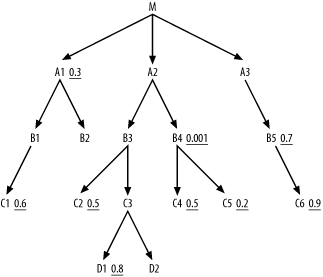
For Step 1, you quickly find that B4 has the best filter ratio, at 0.001, so choose that as the driving table. It's best to reach such a selective filter through an index; so, in real life, if this were an important enough query, you might create a new index to use in driving to B4. For now though, we'll just worry about the join order. Step 2 dictates that you next examine the downward-joined nodes C4 and C5, with a preference to join to better-filtered nodes first. C5 has a filter ratio of 0.2, while C4 has a filter ratio of 0.5, so you join to C5 next. At this point, the beginning join order is (B4, C5), and the cloud around the so-far-joined tables looks like Figure 6-5.
Figure 6-5. So-far-joined cloud, with two tables joined
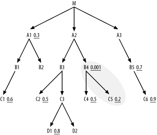
If C5 had one or more nodes connected below, you would now have to compare them to C4, but since it does not, Step 2 offers only the single choice of C4. When you widen the cloud boundaries to include C4, you find no further nodes below the cloud, so you move on to Step 3, find the single node A2 joining the cloud from above, and add it to the building join order, which is now (B4, C5, C4, A2). The cloud around the so-far-joined tables now looks like Figure 6-6.
Figure 6-6. So-far-joined cloud, after four tables joined
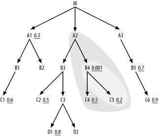
Note that I left in the original two-node cloud in gray. In practice, you need not erase the earlier clouds; just redraw new clouds around them. Returning to Step 2, find downstream of the current joined-tables cloud a single node, B3, so put it next in the join order without regard to any filter ratio it might have. Extend the cloud boundaries to include B3, so you now find nodes C2 and C3 applicable under Step 2, and choose C2 next in the join order, because its filter ratio of 0.5 is better than the implied filter ratio of 1.0 on unfiltered C3. The join order so far is now (B4, C5, C4, A2, B3, C2). Extend the cloud further around C2. This brings no new downstream nodes into play, so Step 2 now offers only C3 as an alternative. The join order so far is now (B4, C5, C4, A2, B3, C2, C3), and Figure 6-7 shows the current join cloud.
Figure 6-7. So-far-joined cloud, with seven tables joined
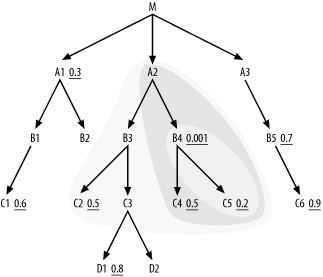
Step 2 now offers two new nodes below the current join cloud, D1 and D2, with D1 offering the better filter ratio. Since neither of these has nodes joined below, join to them in filter-ratio order and proceed to Step 3, with the join order so far now (B4, C5, C4, A2, B3, C2, C3, D1, D2). This completes the entire branch from A2 down, leaving only the upward link to M (the main table being queried) to reach the rest of the join tree, so Step 3 takes you next to M. Since you have reached the main table at the root of the join tree, Step 3 does not apply for the rest of the problem. Apply Step 2 until you have reached the rest of the tables. Immediately downstream of M (and of the whole join cloud so far), you find A1 and A3, with only A1 having a filter, so you join to A1 next. Now, the join order so far is (B4, C5, C4, A2, B3, C2, C3, D1, D2, M, A1), and Figure 6-8 shows the current join cloud.
Figure 6-8. So-far-joined cloud, with 11 tables joined
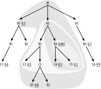
Find immediately downstream of the join cloud nodes B1, B2, and A3, but none of these have filters, so look for two-away filters that offer the best filter ratios two steps away. You find such filters on C1 and B5, but C1 has the best, so add B1 and C1 to the running join order. Now, the join order so far is (B4, C5, C4, A2, B3, C2, C3, D1, D2, M, A1, B1, C1). You still find no better prospect than the remaining two-away filter on B5, so join next to A3 and B5, in that order. Now, the only two nodes remaining, B2 and C6, are both eligible to join next, being both directly attached to the join cloud. Choose C6 first, because it has a filter ratio of 0.9, which is better than the implied filter ratio of 1.0 for the unfiltered join to B2. This completes the join order:(B4, C5, C4, A2, B3, C2, C3, D1, D2, M, A1, B1, C1, A3, B5, C6, B2).
Apart from the join order, the rules specify that the database should reach table B4 on the index for its filter condition and the database should reach all the other tables in nested loops to the indexes on their join keys. These indexed join keys would be primary keys for downward joins to C5, C4, B3, C2, C3, D1, D2, A1, B1, C1, A3, B5, C6, and B2, and foreign keys for A2 (pointing to B4) and M (pointing to A2). Taken together, this fully specifies a single optimum robust plan out of the 17-factorial (355,687,428,096,000) possible join orders and all possible join methods and indexes. However, this example is artificial in two respects:
Real queries rarely have so many filtered nodes, so it is unlikely that a join of so many tables would have a single optimum join order. More commonly, there will be a whole range of equally good join orders, as I showed in the previous example.
The later part of the join order matters little to the runtime, as long as you get the early join order right and reach all the later tables through their join keys. In this example, once the database reached node M, and perhaps A1, with the correct path, the path to the rest of the tables would affect the query runtime only slightly. In most queries, even fewer tables really matter to the join order, and often you will do fine with just the correct driving table and nested loops to the other tables following join keys in any order that the join tree permits.
|


