7.2 Queries with Subqueries

Almost all real-world queries with subqueries impose a special kind of condition on the rows in the outer, main query; they must match or not match corresponding rows in a related query. For example, if you need data about departments that have employees, you might query:

SELECT ... 
FROM Departments D 
WHERE EXISTS (SELECT NULL 
              FROM Employees E
              WHERE E.Department_ID=D.Department_ID)

Alternatively, you might query for data about departments that do not have employees:

SELECT ... FROM Departments D
WHERE NOT EXISTS (SELECT NULL 
                  FROM Employees E
                  WHERE E.Department_ID=D.Department_ID)

The join E.Department_ID=D.Department_ID in each of these queries is the correlation join, which matches between tables in the outer query and the subquery. The EXISTS query has an alternate, equivalent form:

SELECT ... 
FROM Departments D
WHERE D.Department_ID IN (SELECT E.Department_ID FROM Employees E)

Since these forms are functionally equivalent, and since the diagram should not convey a preconceived bias toward one form or another, both forms result in the same diagram. Only after evaluating the diagram to solve the tuning problem should you choose which form best solves the tuning problem and expresses the intended path to the data.

7.2.1 Diagramming Queries with Subqueries

Ignoring the join that links the outer query with the subquery, you can already produce separate, independent query diagrams for each of the two queries. The only open question is how you should represent the relationship between these two diagrams, combining them into a single diagram. As the EXISTS form of the earlier query makes clear, the outer query links to the subquery through a join: the correlation join. This join has a special property: for each outer-query row, the first time the database succeeds in finding a match across the join, it stops looking for more matches, considers the EXISTS condition satisfied, and passes the outer-query row to the next step in the execution plan. When it finds a match for a NOT EXISTS correlated subquery, it stops with the NOT EXISTS condition that failed and immediately discards the outer-query row, without doing further work on that row. All this behavior suggests that a query diagram should answer four special questions about a correlation join, questions that do not apply to ordinary joins:

Is it an ordinary join? (No, it is a correlation join to a subquery.)
Which side of the join is the subquery, and which side is the outer query?
Is it expressible as an EXISTS or as a NOT EXISTS query?
How early in the execution plan should you execute the subquery?

When working with subqueries and considering these questions, remember that you still need to convey the properties you convey for any join: which end is the master table and how large are the join ratios.

7.2.1.1 Diagramming EXISTS subqueries

Figure 7-27 shows my convention for diagramming a query with an EXISTS-type subquery (which might be expressed by the equivalent IN subquery). The figure is based on the earlier EXISTS subquery:

SELECT ... FROM Departments D
WHERE EXISTS (SELECT NULL 
              FROM Employees E 
              WHERE E.Department_ID=D.Department_ID)

Figure 7-27. A simple query with a subquery

For the correlation join (known as a semi-join when applied to an EXISTS-type subquery) from Departments to Employees, the diagram begins with the same join statistics shown for Figure 5-1.

Like any join, the semi-join that links the inner query to the outer query is a link with an arrowhead on any end of the join that points toward a primary key. Like any join link, it has join ratios on each end, which represent the same statistical properties the same join would have in an ordinary query. I use a midpoint arrow to point from the outer-query correlated node to the subquery correlated node. I place an E beside the midpoint arrow to show that this is a semi-join for an EXISTS or IN subquery.

In this case, as in many cases with subqueries, the subquery part of the diagram is a single node, representing a subquery without joins of its own. Less frequently, also as in this case, the outer query is a single node, representing an outer query with no joins of its own. The syntax is essentially unlimited, with the potential for multiple subqueries linked to the outer query, for subqueries with complex join skeletons of their own, and even for subqueries that point to more deeply nested subqueries of their own.

The semi-join link also requires up to two new numbers to convey properties of the subquery for purposes of choosing the best plan. Figure 7-27 shows both potential extra values that you sometimes need to choose the optimum plan for handling a subquery.

The first value, next to the E (20 in Figure 7-27) is the correlation preference ratio. The correlation preference ratio is the ratio of I/E. E is the estimated or measured runtime of the best plan that drives from the outer query to the subquery (following EXISTS logic). I is the estimated or measured runtime of the best plan that drives from the inner query to the outer query (following IN logic). You can always measure this ratio directly by timing both forms, and doing so is usually not much trouble, unless you have many subqueries combined. Soon I will explain some rules of thumb to estimate I/E more or less accurately, and even a rough estimate is adequate to choose a plan when, as is common, the value is either much less than 1.0 or much greater than 1.0. When the correlation preference ratio is greater than 1.0, choose a correlated subquery with an EXISTS condition and a plan that drives from the outer query to the subquery.

The other new value is the subquery adjusted filter ratio (0.8 in Figure 7-27), next to the detail join ratio. This is an estimated value that helps you choose the best point in the join order to test the subquery condition. This applies only to queries that should begin with the outer query, so exclude it from any semi-join link (with a correlation preference ratio less than 1.0) that you convert to the driving query in the plan.

If you have more than one semi-join with a correlation preference ratio less than 1.0, you will drive from the subquery with the lowest correlation preference ratio, and you still need adjusted filter ratios for the other subqueries.

Before I explain how to calculate the correlation preference ratio and the subquery adjusted filter ratios, let's consider when you even need them. Figure 7-28 shows a partial query diagram for an EXISTS-type subquery, with the root detail table of the subquery on the primary-key end of the semi-join.

Figure 7-28. A semi-join to a primary key

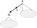
Here, the semi-join is functionally no different than an ordinary join, because the query will never find more than a single match from table M for any given row from the outer query.

I assume here that the whole subtree under M is normal-form (i.e., with all join links pointing downward toward primary keys), so the whole subquery maps one-to-one with rows from the root detail table M of the subtree.

Since the semi-join is functionally no different than an ordinary join, you can actually buy greater degrees of freedom in the execution plan by explicitly eliminating the EXISTS condition and merging the subquery into the outer query. For example, consider this query:

SELECT <Columns from outer query only>
FROM Order_Details OD, Products P, Shipments S, 
     Addresses A, Code_Translations ODT
WHERE OD.Product_ID = P.Product_ID
  AND P.Unit_Cost > 100
  AND OD.Shipment_ID = S.Shipment_ID
  AND S.Address_ID = A.Address_ID(+)
  AND OD.Status_Code = ODT.Code
  AND ODT.Code_Type = 'Order_Detail_Status'
  AND S.Shipment_Date > :now - 1
  AND EXISTS (SELECT null
              FROM Orders O, Customers C, Code_Translations OT, 
                   Customer_Types CT
              WHERE C.Customer_Type_ID = CT.Customer_Type_ID
                AND CT.Text = 'Government'
                AND OD.Order_ID = O.Order_ID
                AND O.Customer_ID = C.Customer_ID
                AND O.Status_Code = OT.Code
                AND O.Completed_Flag = 'N'
                AND OT.Code_Type = 'ORDER_STATUS'
                AND OT.Text != 'Canceled')
ORDER BY <Columns from outer query only>

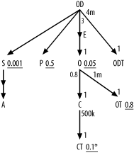
Using the new semi-join notation, you can diagram this as shown in Figure 7-29.

Figure 7-29. A complex example of a semi-join with a correlation to the primary key of the subquery root detail table

If you simply rewrite this query to move the table joins and conditions in the subquery into the outer query, you have a functionally identical query, since the semi-join is toward the primary key and the subquery is one-to-one with its root detail table:

SELECT <Columns from the original outer query only>
FROM Order_Details OD, Products P, Shipments S, 
     Addresses A, Code_Translations ODT,
     Orders O, Customers C, Code_Translations OT, Customer_Types CT
WHERE OD.Product_Id = P.Product_Id
  AND P.Unit_Cost > 100
  AND OD.Shipment_Id = S.Shipment_Id
  AND S.Address_Id = A.Address_Id(+)
  AND OD.Status_Code = ODT.Code
  AND ODT.Code_Type = 'Order_Detail_Status'
  AND S.Shipment_Date > :now - 1
                AND C.Customer_Type_Id = CT.Customer_Type_Id
                AND CT.Text = 'Government'
                AND OD.Order_Id = O.Order_Id
                AND O.Customer_Id = C.Customer_Id
                AND O.Status_Code = OT.Code
                AND O.Completed_Flag = 'N'
                AND OT.Code_Type = 'ORDER_STATUS'
                AND OT.Text != 'Canceled'
ORDER BY <Columns from the original outer query only>

I have indented this version to make obvious the simple transformation from one to the other in this case. The query diagram is also almost identical, as shown in Figure 7-30.

Figure 7-30. The same query transformed to merge the subquery

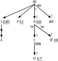
This new form has major additional degrees of freedom, allowing, for example, a plan joining to moderately filtered P after joining to highly filtered O but before joining to the almost unfiltered node OT. With the original form, the database would be forced to complete the whole subquery branch before it could consider joins to further nodes of the outer query. Since merging the subquery in cases like this can only help, and since this creates a query diagram you already know how to optimize, I will assume for the rest of this section that you will merge this type of subquery. I will only explain diagramming and optimizing other types.

In theory, you can adapt the same trick for merging EXISTS-type subqueries with the semi-join arrow pointing to the detail end of the join too, but it is harder and less likely to help the query performance. Consider the earlier query against departments with the EXISTS condition on Employees:

SELECT ... 
FROM Departments D
WHERE EXISTS (SELECT NULL 
              FROM Employees E 
              WHERE E.Department_ID=D.Department_ID)

These are the problems with the trick in this direction:

The original query returns at most one row per master table row per department. To get the same result from the transformed query, with an ordinary join to the detail table (Employees), you must include a unique key of the master table in the SELECT list and perform a DISTINCT operation on the resulting query rows. These steps discard duplicates that result when the same master record has multiple matching details.
When there are several matching details per master row, it is often more expensive to find all the matches than to halt a semi-join after finding just the first match.

Therefore, you should rarely transform semi-joins to ordinary joins when the semi-join arrow points upward, except when the detail join ratio for the semi-join is near 1.0 or even less than 1.0.

To complete a diagram for an EXISTS-type subquery, you just need rules to estimate the correlation preference ratio and the subquery adjusted filter ratio. Use the following procedure to estimate the correlation preference ratio:

For the semi-join, let D be the detail join ratio, and let M be the master join ratio. Let S be the best (smallest) filter ratio of all the nodes in the subquery, and let R be the best (smallest) filter ratio of all the nodes in the outer query.
If D x S<M / R, set the correlation preference ratio to (D x S)/(M x R).
Otherwise, if S>R, set the correlation preference ratio to S/R.

Otherwise, let E be the measured runtime of the best plan that drives from the outer query to the subquery (following EXISTS logic). Let I be the measured runtime of the best plan that drives from the inner query to the outer query (following IN logic). Set the correlation preference ratio to I/E. When Steps 2 or 3 find an estimate for the correlation preference ratio, you are fairly safe knowing which direction to drive the subquery without measuring actual runtimes.

The estimated value from Step 2 or Step 3 might not give the accurate runtime ratio you could measure. However, the estimate is adequate as long as it is conservative, avoiding a value that leads to an incorrect choice between driving from the outer query or the subquery. The rules in Steps 2 and 3 are specifically designed for cases in which such safe, conservative estimates are feasible.

When Steps 2 and 3 fail to produce an estimate, the safest and easiest value to use is what you actually measure. In this range, which you will rarely encounter, finding a safe calculated value would be more complex than is worth the trouble.

Once you have found the correlation preference ratio, check whether you need the subquery adjusted filter ratio and determine the subquery adjusted filter ratio when you need it:

If the correlation preference ratio is less than 1.0 and less than all other correlation preference ratios (in the event that you have multiple subqueries), stop. In this case, you do not need a subquery preference ratio, because it is helpful only when you're determining when you will drive from the outer query, which will not be your choice.
If the subquery is a single-table query with no filter condition, just the correlating join condition, measure q (the rowcount with of the outer query with the subquery condition removed) and t (the rowcount of the full query, including the subquery). Set the subquery adjusted filter ratio to t/q. (In this case, the EXISTS condition is particularly easy to check: the database just looks for the first match in the join index.)
Otherwise, for the semi-join, let D be the detail join ratio. Let s be the filter ratio of the correlating node (i.e., the node attached to the semi-join link) on the detail, subquery end.
If D 1, set the subquery adjusted filter ratio equal to s / D.
Otherwise, if s x D<1, set the subquery adjusted filter ratio equal to (D-1+(s x D))/D.
Otherwise, set the subquery adjusted filter ratio equal to 0.99. Even the poorest-filtering EXISTS condition will avoid actually multiplying rows and will offer a better filtering power per unit cost than a downward join with no filter at all. This last rule covers these better-than-nothing (but not much better) cases.

Like other rules in this book, the rules for calculating the correlation preference ratio and the subquery adjusted filter ratio are heuristic. Because exact numbers are rarely necessary to choose the right execution plan, this carefully designed, robust heuristic leads to exactly the right decision at least 90% of the time and almost never leads to significantly suboptimal choices. As with many other parts of this book, a perfect calculation for a complex query would be well beyond the scope of a manual tuning method.

Try to see if you understand the rules to fill in the correlation preference ratio and the subquery adjusted filter ratio by completing Figure 7-31, which is missing these two numbers.

Figure 7-31. A complex query with missing values for the semi-join

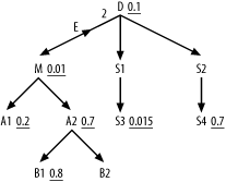
Check your own work against this explanation. Calculate the correlation preference ratio:

Set D=2 and M=1 (implied by its absence from the diagram). Set S=0.015 (the best filter ratio of all those in the subquery, on the table S3, which is two levels below the subquery root detail table D). Then set R=0.01, which is the best filter for any node in the tree under and including the outer-query's root detail table M.
Find D x S=0.03 and M x R=0.01, so D / S>M x R. Move on to Step 3.
Since S>R, set the correlation preference ratio to S/R, which works out to 1.5.

To find the subquery adjusted filter ratio, follow these steps:

Note that the correlation preference ratio is greater than 1, so you must proceed to Step 2.
Note that the subquery involves multiple tables and contains filters, so proceed to Step 3.
Find D=2, and find the filter ratio on node D, s=0.1.
Note that D>1, so proceed to Step 5.
Calculate s x D=0.2, which is less than 1, so you estimate the subquery adjusted filter ratio as (D-1+(s x D))/D = (2-1+(0.1 x 2))/2 = 0.6.

In the following section on optimizing EXISTS subqueries, I will illustrate optimizing the completed diagram, shown in Figure 7-32.

7.2.1.2 Diagramming NOT EXISTS subqueries

Subquery conditions that you can express with NOT EXISTS or NOT IN are simpler than EXISTS-type subqueries in one respect: you cannot drive from the subquery outward to the outer query. This eliminates the need for the correlation preference ratio. The E that indicates an EXISTS-type subquery condition is replaced by an N to indicate a NOT EXISTS-type subquery condition, and the correlation join is known as an anti-join rather than a semi-join, since it searches for the case when the join to rows from the subquery finds no match.

It turns out that it is almost always best to express NOT EXISTS-type subquery conditions with NOT EXISTS, rather than with NOT IN. Consider the following template for a NOT IN subquery:

SELECT ... 
FROM ... Outer_Anti_Joined_Table Outer 
WHERE...
  AND Outer.Some_Key NOT IN (SELECT Inner.Some_Key 
                             FROM ... Subquery_Anti_Joined_Table Inner WHERE 
                             <Conditions_And_Joins_On_Subquery_Tables_Only>)
...

You can and should rephrase this in the equivalent NOT EXISTS form:

SELECT ... 
FROM ... Outer_Anti_Joined_Table Outer 
WHERE...
  AND Outer.Some_Key IS NOT NULL
  AND NOT EXISTS (SELECT null 
                  FROM ... Subquery_Anti_Joined_Table Inner WHERE 
                  <Conditions_And_Joins_On_Subquery_Tables_Only>
                  AND Outer.Some_Key = Inner.Some_Key)

To convert NOT IN to NOT EXISTS without changing functionality, you need to add a not-null condition on the correlation join key in the outer table. This is because the NOT IN condition amounts to a series of not-equal-to conditions joined by OR, but a database does not evaluate NULL!=<SomeValue> as true, so the NOT IN form rejects all outer-query rows with null correlation join keys. This fact is not widely known, so it is possible that the actual intent of such a query's developer was to include, in the query result, these rows that the NOT IN form subtly excludes. When you convert forms, you have a good opportunity to look for and repair this likely bug.

Both EXISTS-type and NOT EXISTS-type subquery conditions stop looking for matches after they find the first match, if one exists. NOT EXISTS subquery conditions are potentially more helpful early in the execution plan, because when they stop early with a found match, they discard the matching row, rather than retain it, making later steps in the plan faster. In contrast, to discard a row with an EXISTS condition, the database must examine every potentially matching row and rule them all out, a more expensive operation when there are many details per master across the semi-join. Remember the following rules, which compare EXISTS and NOT EXISTS conditions that point to detail tables from a master table in the outer query:

An unselective EXISTS condition is inexpensive to check (since it finds a match easily, usually on the first semi-joined row it checks) but rejects few rows from the outer query. The more rows the subquery, isolated, would return, the less expensive and the less selective the EXISTS condition is to check. To be selective, an EXISTS condition will also likely be expensive to check, since it must rule out a match on every detail row.
A selective NOT EXISTS condition is inexpensive to check (since it finds a match easily, usually on the first semi-joined row it checks) and rejects many rows from the outer query. The more rows the subquery, isolated, would return, the less expensive and the more selective the EXISTS condition is to check. On the other hand, unselective NOT EXISTS conditions are also expensive to check, since they must confirm that there is no match for every detail row.

Since it is generally both more difficult and less rewarding to convert NOT EXISTS subquery conditions to equivalent simple queries without subqueries, you will often use NOT EXISTS subqueries at either end of the anti-join: the master-table end or the detail-table end. You rarely need to search for alternate ways to express a NOT EXISTS condition.

Since selective NOT EXISTS conditions are inexpensive to check, it turns out to be fairly simple to estimate the subquery adjusted filter ratio:

Measure q (the rowcount of the outer query with the NOT EXISTS subquery condition removed) and t (the rowcount of the full query, including the subquery). Let C be the number of tables in the subquery FROM clause (usually one, for NOT EXISTS conditions).
Set the subquery adjusted filter ratio to (C-1+(t/q))/C.

7.2.2 Tuning Queries with Subqueries

As for simple queries, optimizing complex queries with subqueries turns out to be straightforward, once you have a correct query diagram. Here are the steps for optimizing complex queries, including subqueries, given a complete query diagram:

Convert any NOT IN condition into the equivalent NOT EXISTS condition, following the earlier template.
If the correlation join is an EXISTS-type join, and the subquery is on the master end of that join (i.e., the midpoint arrow points down), convert the complex query to a simple query as shown earlier, and tune it following the usual rules for simple queries.
Otherwise, if the correlation join is an EXISTS-type join, find the lowest correlation preference ratio of all the EXISTS-type subqueries (if there is more than one). If that lowest correlation preference ratio is less than 1.0, convert that subquery condition to the equivalent IN condition and express any other EXISTS-type subquery conditions using the EXISTS condition explicitly. Optimize the noncorrelated IN subquery as if it were a standalone query; this is the beginning of the execution plan of the whole query. Upon completion of the noncorrelated subquery, the database will perform a sort operation to discard duplicate correlation join keys from the list generated from the subquery. The next join after completing this first subquery is to the correlating key in the outer query, following the index on that join key, which should be indexed. From this point, treat the outer query as if the driving subquery did not exist and as if this first node were the driving table of the outer query.
If all correlation preference ratios are greater than or equal to 1.0, or if you have only NOT EXISTS-type subquery conditions, choose a driving table from the outer query as if that query had no subquery conditions, following the usual rules for simple queries.
As you reach nodes in the outer query that include semi-joins or anti-joins to not-yet-executed subqueries, treat each entire subquery as if it were a single, downward-hanging node (even if the correlation join is actually upward). Choose when to execute the remaining subqueries as if this virtual node had a filter ratio equal to the subquery adjusted filter ratio.

Because correlated subqueries stop at the first row matched, if any, they avoid the row-multiplying risk of normal upward joins and can only reduce the running rowcount. However, since they must often examine many rows to have this filtering effect, the correct value of the subquery adjusted filter ratio often makes this virtual node equivalent to an almost unfiltered node in benefit/cost ratio.

Wherever you place the correlated join in the join order following Step 5, you then immediately perform the rest of that correlated subquery, optimizing the execution plan of that subquery with the correlating node as the driving node of that independent query. When finished with that subquery, return to the outer query and continue to optimize the rest of the join order.

As an example, consider Figure 7-32, which is Figure 7-31 with the correlation preference ratio and the subquery adjusted filter ratio filled in.

Figure 7-32. Example problem optimizing a complex query with a subquery

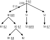
Since the correlated join is EXISTS-type, Step 1 does not apply. Since the midpoint arrow of the semi-join points upward, Step 2 does not apply. The lowest (the only) correlation preference ratio is 1.5 (next to the E), so Step 3 does not apply. Applying Step 4, you find that the best driving node in the outer query is M. Applying Step 5, choose between downward joins to A1 and A2 with filter ratios of 0.2 and 0.7, respectively, or a virtual downward join to the virtual node representing the whole subquery, with a virtual filter ratio of 0.6. A1 is the best of these three candidates, with the best filter ratio, so join to it next. Finding nothing downstream of A1, you next find the subquery as the next-best choice in the join order (again applying Step 5), so perform the semi-join to D.

Applying Step 6, having begun the subquery, you must finish it, starting from D as the driving node. Following simple-query rules within that subquery, next join to S1, S3, S2, and S4, in that order. Returning to the outer query, applying the usual rules for simple queries, you find the remainder of the join order, A2, B1, B2. The whole optimum join order, including the semi-join, is then (M, A1, D, S1, S3, S2, S4, A2, B1, B2).

Must You Worry About Subqueries?

The rules for subqueries are complex enough to be discouraging, so I'd like to offer a confession that might help your morale. For over 10 years, I've successfully tuned SQL with subqueries without using formal rules, following intuition and a general rule to choose between driving from the subquery or the outer query based on which had the most selective conditions. I don't usually worry much about when subqueries execute, except when they should actually drive the query, since this is usually hard to control and improvements versus the optimizers' automatic choices are usually minor.

I occasionally (less often than you might think, though) recognize borderline cases in which it makes sense to try multiple alternatives and choose the fastest. The same approach might work for you as well. If you mistrust intuition or want a basis for it that incorporates my own experience, you will find the formal rules useful. The formal rules of this section, which I worked out specifically for this book, handle the full range of realistic queries with a reasonable compromise between mathematical perfection and usability. Only massive brute-force calculation can handle the full complexity of the problem perfectly without trial and error, but these rules offer a sort of automated intuition, if you will, that is at least as good as my old seat-of-the-pants approach.