A.1 Chapter 5 Exercise Solutions

Following are the solutions to the exercises in Section 5.5.

A.1.1 Exercise 1

Figure A-1 shows the solution to Exercise 1.

Figure A-1. Solution to Exercise 1

The subtlest aspect of this exercise is that you need to notice that you do not need queries (other than the total table rowcounts) to find the filter ratios for the R and D nodes. From the exact matches on uniquely indexed names for each of these, a single match for R and an IN list for D, you can deduce the ratios. You just need to calculate 1/R and 2/D, where D and R are the respective rowcounts of those tables, to find their filter ratios. Did you remember to add the * to the filter ratio on R to indicate that it turns out to be a unique condition? (This turns out to be important for optimizing some queries!) You would add an asterisk for the condition on D, as well, if the match were with a single name instead of a list of names.

The other trick to notice is that, by the assumption of never-null foreign keys with perfect referential integrity, the rowcounts of the joins would simply equal the rowcounts of the detail tables. Therefore, the detail join ratios are simply d/m, where d is the rowcount of the upper detail table and m is the rowcount of the lower master table. The master join ratios under the same assumptions are exactly 1.0, and you simply leave them off.

A.1.2 Exercise 2

Figure A-2 shows the solution to Exercise 2.

Figure A-2. Solution to Exercise 2

In this problem, you need the same shortcuts as for Exercise 1, for join ratios and for the filter ratio to B. Did you remember to add the * for the unique filter on B? Did you remember to indicate the direction of the outer joins to Z and R with the midpoint arrows on those join links?

A.1.3 Exercise 3

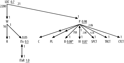
Figure A-3 shows the solution to Exercise 3.

Figure A-3. Solution to Exercise 3

In this problem, you need the same tricks as for Exercise 1, for join ratios and for the filter ratio to B. Did you remember to add the * for the unique filter on B? Did you remember to indicate the direction of the outer joins to C and PL with the midpoint arrows on those join links?

The joins to ITxR and IV from ITx and P, respectively, are special one-to-one joins that you indicate with arrows on both ends of the join links. The filter ratios on both ends of these one-to-one joins are exactly 1.0. These are a special class of detail table that frequently comes up in real-world applications: time-dependent details that have one row per master row corresponding to any given effective date. For example, even though you might have multiple inventory tax rates for a given taxing entity, only one of those rates will be in effect at any given moment, so the date ranges defined by Effective_Start_Date and Effective_End_Date will be nonoverlapping. Even though the combination of ID and date-range condition do not constitute equality conditions on a full unique key, the underlying valid data will guarantee that the join is unique when it includes the date-range conditions.

Since you count the date range defined by Effective_Start_Date and Effective_End_Date as part of the join, do not count it as a filter, and consider only the subtable that meets the date-range condition as effective for the query diagram. Thus, you find P and IV to have identical effective rowcounts of 8,500, and you find identical rowcounts of 4 for ITx and ITxR. This confirms the one-to-one nature of these joins and the join ratios of 1.0 on each end of the links.

As for the example in Figure 5-4, you should use only subtable rowcounts for the joins to SPCT, TRCT, and CTCT, because Code_Translations is one of those apples-and-oranges tables that join only a specific subtable at a time.

I have relaxed my own rule about showing just a single significant figure in the join and filter ratios. This is largely just to help you see that you really have made the right calculations; you haven't just hit the right number for the wrong reason.

A.1.4 Exercise 4

Figure A-4 shows the solution to Exercise 4, the fully simplified solution to Exercise 1.

Figure A-4. Solution to Exercise 4

Since this problem involves only large detail join ratios and master join ratios equal to 1.0, you just add a capital F to the most highly filtered node and add a lowercase f to the other filtered nodes, with an asterisk for the unique filter on node R. (Did you remember the asterisk?)

A.1.5 Exercise 5

Figure A-5 shows the solution to Exercise 5, the fully simplified solution to Exercise 2.

Figure A-5. Solution to Exercise 5

Since this problem involves only large detail join ratios, and master join ratios equal to 1.0, you just add a capital F to the most highly filtered node and add a lowercase f to the other filtered node, with an asterisk for the unique filter on node B. (Did you remember the asterisk?)

A.1.6 Exercise 6

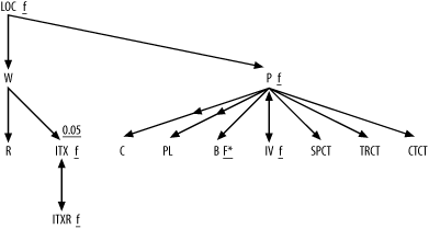
Figure A-6 shows the solution to Exercise 6, the fully simplified solution to Exercise 3.

Figure A-6. Solution to Exercise 6

Since this problem involves only large detail join ratios, you can leave those out. However, note that it does include one master join ratio well under 1.0, in the join down into ITx, so you leave that one in. Otherwise, you just add a capital F to the most highly filtered node and add a lowercase f to the other filtered nodes, with an asterisk for the unique filter on node B. (Did you remember the asterisk?)