6.5 A Complex Example

Now, I demonstrate an example that delivers a less straightforward join order that requires more attention to the whole join cloud. You will find that the sequence of next-best tables can jump all over the query diagram in cases like the one I describe in this section. Consider the problem in Figure 6-9, and try it yourself before you read on.

Figure 6-9. Another problem with the same join skeleton

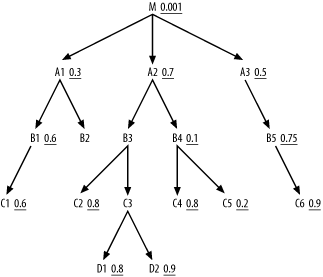
Here, you see, as is quite common, that the best filter falls on the root detail table.

The best filter is often on the root detail table, because the entities of this table are the true focus of the query. It is common that the main filter references a direct property of those entities, rather than some inherited property in the joined tables.

Since you will drive from the root detail table, Step 3 will never apply; you have no nodes upstream of the starting point. The cloud of tables joined so far will grow downward from the top, but keep in mind that you can find the next-best node anywhere along the boundary of this cloud, not necessarily near the last table joined. Try to find the best join order yourself before you read on.

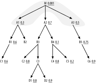
The first eligible nodes are A1, A2, and A3, and the best filter ratio lies on A1, so A1 falls second in the join order. After extending the join cloud to A1, add B1 and B2 to the eligible nodes, and A2 and A3 are still eligible. Between these four nodes, A3 has the best filter ratio, so join to it next. The join order, so far, is (M, A1, A3), and the join cloud now looks like Figure 6-10.

Figure 6-10. Join cloud after the first three tables

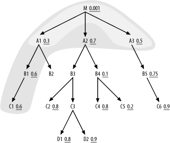
The list of eligible nodes attached to the join cloud is now B1, B2, A2, and B5. B1 has the best filter ratio among these, so join to it next, extending the cloud and adding C1 to the list of eligible nodes, which is now B2, A2, B5, and C1. Among these, C1 is the best, so join to it next and extend the cloud further. C1 has no downstream nodes, so proceed to the next-best node on the current list, A2, which adds B3 and B4 to the list of eligible nodes, which is now B2, B5, B3, and B4. The join order, so far, is (M, A1, A3, B1, C1, A2), and the join cloud now looks like Figure 6-11.

Figure 6-11. Join cloud after the first six tables

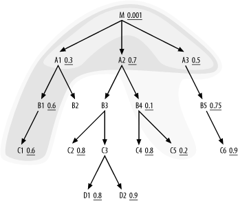
Among the eligible nodes, B4 has, by far, the best filter ratio, so it comes next. (It would have been great to join to it earlier, but it did not become eligible until the database reached A2.) The join order to B4 adds C4 and C5 to the eligible list, which now includes B2, B5, B3, C4, and C5. Of these, C5 is by far the best, so it comes next. The join order, so far, is (M, A1, A3, B1, C1, A2, B4, C5), and the join cloud now looks like Figure 6-12.

Figure 6-12. Join cloud after the first eight tables

Eligible nodes attached below the join cloud now include B2, B3, B5, and C4, and the best filter among these is B5. B5 adds C6 to the eligible list, and the next-best on the list is C4, which adds no new node to the list. C6 is the next-best node, but it also adds no new node to the eligible-nodes list, which is now just B2 and B3. Neither of these even has a filter, so you look for two-away filters and find that B3 at least gives access to the filter on C2, so you join to B3 next. The join order, so far, is (M, A1, A3, B1, C1, A2, B4, C5, B5, C4, C6, B3), and the join cloud now looks like Figure 6-13.

Figure 6-13. Join cloud after the first 12 tables

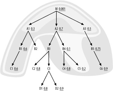
You now find eligible nodes B2, C2, and C3, and only C2 has a filter, so join to C2 next. It has no downstream node, so choose between B2 and C3 and again use the tiebreaker that C3 at least gives access to two-away filters on D1 and D2, so join C3 next. The join order, so far, is now (M, A1, A3, B1, C1, A2, B4, C5, B5, C4, C6, B3, C2, C3). The eligible downstream nodes are now B2, D1, and D2. At this point in the process, the eligible downstream nodes are the only nodes left, having no nodes further downstream. Just sort the nodes left by filter ratio, and complete the join order: (M, A1, A3, B1, C1, A2, B4, C5, B5, C4, C6, B3, C2, C3, D1, D2, B2). In real queries, you usually get to the point of just sorting immediately attached nodes sooner. In the common special case of a single detail table with only direct joins to master-table lookups (dimension tables, usually), called a star join, you sort master nodes right from the start.

Given the optimal order just derived, complete the specification of the execution plan by calling for access to the driving table M from an index for the filter condition on that table. Then join the other tables using nested loops joins that follow indexes on those tables' primary keys.

Driving from the root node of the join tree is particularly simple, since you can usually count on finding indexes already in place for the primary keys the database needs to join exclusively in the downward direction.