15.2 Past Work

   

---

The ideas illustrated in this chapter originate from past work on the integration of database technology and data-mining tools, and from the notion of an inductive database. In order to make clear our proposal, it is necessary to report this past work, showing the background that inspired our present work. In particular, we will consider two main data-mining problems: the association rule extraction problem and the classification problem.

15.2.1 Extracting and Evaluating Association Rules

We describe here a classical market basket analysis problem that will serve as a running example throughout the chapter to illustrate association rule mining problems.

We are looking for associations between two sets of items bought by customers in the same purchase transaction, with the purpose of discovering the behavior of customer purchases.

The source database from which association rules might be extracted is shown in Table 15.1.

Association Rules

An association rule is a pair of two sets of items extracted from within purchase transactions. An example of an association rule extracted from the Transactions Table is {A}{B}. A is the antecedent (or body), and B the consequent (or head) of the rule. In Table 15.1, {A}{B} is satisfied by the customer c1, c3, and c4, because both items A and B are bought by those customers in the transactions 1, 3, 4, and 5, respectively. The intuitive meaning of {A}{B} is that the customers that buy A in a transaction also tend to buy B in the same transaction. Association rules are extracted from the database having computed the value of two statistical measures, whose purpose is to give the association rules frequency and statistical relevance.

Support is the statistical frequency with which the association rule is present in the table. It is given by the number of transactions in the source table in which both the sets of items (the antecedent and the consequent) are present, divided by the total number of transactions in the table (in the example of Table 15.1, {A}{B} has support 4/6).

Confidence is the conditional probability with which customers buy, in a transaction, the consequent of the association rule (in the example B), given that the transaction contains the antecedent (A). Confidence may be obtained by the ratio between the number of transactions containing both the antecedent and the consequent and the number of transactions containing the antecedent. Therefore, in the example of Table 15.1, {A}{B} has confidence 4/5.

The analyst usually specifies minimum values for support and confidence, so that only the most frequent and significant association rules are extracted.

MINE RULE Operator

The purpose of this paragraph is to introduce a running example that will be used to discuss the problem of mining association rules. Therefore this paragraph is not to be considered as a complete overview of the MINE RULE operator. For full details, the reader is directed to (Meo et al. 1998a).

The MINE RULE operator has been introduced with the purpose to request the extraction of association rules from within a relational database, by means of a declarative, SQL-like, query. The problem of extracting the simplest association rules, as described in the preceding paragraph, is specified by the MINE RULE statement in Listing 15.1.

Listing 15.1 MINE RULE Statement

MINE RULE Rule_Set1 AS
SELECT DISTINCT 1..n item AS BODY, 1..1 item AS HEAD
FROM Transactions
GROUP BY transaction_ID
EXTRACTING RULES WITH SUPPORT: 0.5, CONFIDENCE: 0.8

The GROUP BY clause logically partitions the source Transactions table (FROM clause) in groups, such that each group is made by items bought in the same transaction. The SELECT clause selects association rules made by a set of one or more items in the body (1..n item AS BODY), and one single item in the head (1..1 item AS HEAD), coming from the same transaction (group). From all the possible association rules, only those ones that have a support that is at least 0.5 and a confidence at least 0.8 (EXTRACTING clause) are extracted. Finally the extracted association rules, output of the MINE RULE operator, are inserted into a new table, named Rule_Set1. The output of the MINE RULE statement in Listing 15.1 is shown in Table 15.2.

Table 15.2. The Output Table Rule_Set1

Body	Head	Support	Confidence
{A}	{B}	0.667	0.8
{B}	{A}	0.667	0.8
{B}	{C}	0.667	0.8
{C}	{B}	0.667	1
{A,C}	{B}	0.5	1

EVALUATE RULE Operator

If we want to cross over between extracted rules and the original relation, for instance, in order to select the tuples of the source table that satisfy the rules in a given rule set, we need an operator that does the reverse task of the extraction of association rules: It selects the original tuples from the source table for which certain rules hold. A possible operator that does this task is named EVALUATE RULE and has been introduced in Psaila (2001). With this operator, it is also possible to perform aggregations on the rules and other sophisticated operations. Although in this chapter, we consider only a very simple rule evaluation problem, this is still an exemplary instance of the problems that belong to the class of post-processing operations. These are operations, executed after the proper mining operations, that have the purpose of analyzing, with certain detail, the result set of the mining step.

Suppose we want to find those customers for which at least one association rule in the result set Rule_Set1 holds. This problem is expressed by means of the EVALUATE RULE operator in Listing 15.2.

Listing 15.2 EVALUATE RULE Operator

EVALUATE RULE InterestingCustomers AS
SELECT DISTINCT customer, BODY, HEAD
USING RULES Rule_Set1
ASSOCIATING item AS BODY, item AS HEAD
FROM Transactions
GROUP BY customer
DIVIDE BY transaction

From table Transactions (FROM clause), the EVALUATE statement retrieves those customers for which at least an association rule holds in the result set Rule_Set1 (clause USING RULES). Furthermore, for those customers, it also reports the body and the head of the association rules that hold (clause SELECT DISTINCT customer, BODY, HEAD). Clause ASSOCIATING and clause DIVIDE BY specify, respectively, how association rules have been defined and how they have been extracted from table Transactions; finally, clause GROUP BY specifies that rules are evaluated considering transactions of each single customer. In other words, tuples are grouped by customer, because we want to know for which customer rules hold; then, groups are subdivided by transaction, so that rules are evaluated on these subgroups, a customer separately by other customers. The result set is a table, named InterestingCustomers, which is shown in Table 15.3.

Table 15.3. Table InterestingCustomers, Result of the Operator EVALUATE RULE

Customer	Body	Head
c1	{A}	{B}
c1	{B}	{A}
c1	{B}	{C}
c1	{C}	{B}
c1	{A, C}	{B}
c2	{B}	{C}
c2	{C}	{B}
c3	{A}	{B}
c3	{B}	{A}
c3	{B}	{C}
c3	{C}	{B}
c3	{A, C}	{B}
c4	{A}	{B}
c4	{B}	{A}
c4	{B}	{C}
c4	{C}	{B}
c4	{A, C}	{B}

The reader will notice that in the EVALUATE RULE operator, it is necessary to include some of the clauses of the MINE RULE statement that were used when the association rule set was extracted and stored in the referenced table (Rule_Set1). This is necessary in order to indicate the meaning of the association rules and to ensure consistency between the association rules and the analysis performed on the source data through those rules. Unfortunately, this information is not present in the relational database, since tables are stored without keeping track of the actual statement that generated the table. This means that tables generated by the MINE RULE or the EVALUATE RULE operators are meaningless for a user who has no knowledge of the actual statements that generated those tables. Indeed, the user/analyst is expected to remember the MINE RULE statement that generated the rule set.

This intrinsic limitation of the relational model provides an important observation that constitutes one of the main motivations for the new model based on XML presented in this chapter.

15.2.2 Classifying Data

Another typical data-mining problem is the classification problem. A generic classification problem consists of two distinct phases: the training phase and the test phase. In the training phase, a set of classified data, called training set, is analyzed in order to build a classification model?that is, a model that, based on features appearing in the training set, determines in which cases a given class should be used. For example, the training set might describe data about car insurance applicants. Usually, the risk class of insurance applicants has been established by an expert or is based on historical observations: The classification model says which class to apply, depending on the characteristics of applicants (e.g., age, car type, etc.).

The training phase is then followed by the test phase. In this phase, the classification model built in the previous phase is used to classify new unclassified data. For instance, when new car insurance applicants submit their application form, an automatic system may refer to the classification model and assign the proper risk class to each applicant, depending, for example, on the age and/or the car type.

From the algorithmic point of view, the classification problem has been widely studied in the past, so that several algorithms are available. However, we do not want to focus on algorithms, but on the issue of specifying a classification problem. A possible solution, based on the same idea that inspired the MINE RULE operator, has been introduced by P. L. Lanzi and G. Psaila (Lanzi and Psaila 1999). In this work, an operator able to specify classification problems is proposed. This operator, named MINE CLASSIFICATION, is based on the relational model: It operates on relational tables and is based on an SQL-like syntax. We now give a brief description of this operator.

Training Phase

Suppose we want to obtain a classification model from a sample training set for the car insurance application domain. The training set might be the one contained in the table Training_Set, reported in Table 15.4.

This is a very simple training set, in which attributes AGE and CAR-TYPE are the features that characterize applicants, while attribute RISK is the class label. This attribute can assume only two values, "Low" and "High," meaning that we consider only two risk classes.

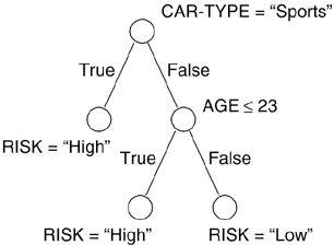
The classification model that can be produced analyzing this training set is basically represented in two distinct, yet equivalent formats: a classification tree or a classification rule set. The classification tree for our case is depicted in Figure 15.1. Nonleaf nodes are labeled with a condition: If the condition is evaluated to true, the branch labeled with "True" is followed; otherwise, the branch labeled with "False" is followed. When a leaf node is reached, it assigns a value to the class. For example, if an applicant owns a truck and is 18 years old, the condition evaluated in the root node is false, and therefore the false branch is followed. Then the condition in the following node (AGE<=23) is evaluated. Being true, it leads to a leaf node with the High value assigned to the Risk class.

Figure 15.1. The Classification Tree Obtained by the Classification Task

Table 15.4. The Table Training_Set, Containing the Training Set for the Classification Process

Age	Car-type	Risk
17	Sports	High
43	Family	Low
68	Family	Low
32	Truck	Low
23	Family	High
18	Family	High
20	Family	High
45	Sports	High
50	Truck	Low
64	Truck	High
46	Family	Low
40	Family	Low

The same classification model might be described by means of classification rules. A possible rule set corresponding to the classification tree depicted in Figure 15.1 follows:

1. IF AGE 23 THEN RISK IS "High"

2. IF CAR-TYPE = "Sports" THEN RISK IS "High"

3. IF CAR-TYPE IS ("Family", "Truck"} AND AGE > 23 THEN RISK IS "Low"

4. DEFAULT RISK IS "Low"

The numbers preceding each rule denote the order in which the rules are evaluated (from the first rule to the following ones) until a rule is satisfied. If no rule is satisfied, the DEFAULT rule is applied. Observe that the condition part of a rule can contain complex conditions, composed using the logical operators.

The data-mining task that leads to the generation of the classification models can be specified, by means of the MINE CLASSIFICATION operator, as shown in Listing 15.3.

Listing 15.3 MINE CLASSIFICATION Operator

MINE CLASSIFICATION Classification_Model AS
SELECT DISTINCT RULES ID, AGE, CAR-TYPE, CLASS
FROM Training_Set
CLASSIFY BY RISK

The statement in Listing 15.3 can be read as follows. The FROM clause specifies the table containing the training set, in this case named Training_Set. Then the CLASSIFY BY clause indicates that the RISK attribute is used as class label. Finally, the SELECT clause specifies the structure of the output table, named Classification_Model: The first attribute of this table is named ID and is the rule identifier; the second and third attributes (AGE and CAR-TYPE) are the attributes on which the conditions of the classification model (expressed in the nodes of the classification tree) are represented. The fourth and last attribute is the class label.

Although it is possible to represent a classification tree in a table, this representation would be unreadable; the MINE CLASSIFICATION operator generates a tabular representation of a classification rule set, where each row corresponds to a rule. We omit the description of this table since it does not add any particular and useful information for the purposes of the present discussion.

Test Phase

Once the classification model has been generated, it should be used to classify new (unclassified) data. Suppose we have a table named New_Applicants, describing data about a set of new applicants for car insurance (see Table 15.5).

Suppose we want to assign each applicant the proper risk class, based on the previously generated model. In practice, we want to obtain table Classified_Applicants (Table 15.6). This table has been obtained by extending rows in Table 15.5 and adding the risk class, obtained by evaluating the classification model on each single row.

Table 15.5. The Table New_Applicants, Containing Unclassified Data

Name	Age	Car-type
John Smyth	22	Family
Marc Green	60	Family
Laura Fox	35	Sports

Table 15.6. The Table Classified_Applicants, Obtained by Extending Table New_Applicants with Class Labels

Name	Age	Car-type	Risk
John Smyth	22	Family	High
Marc Green	60	Family	Low
Laura Fox	35	Sports	High

By means of the MINE CLASSIFICATION operator, it is possible to specify the test phase as well. Table 15.6 might be obtained by Listing 15.4.

Listing 15.4 Test Phase

MINE CLASSIFICATION TEST Classified_Applicants AS
SELECT DISTINCT *, CLASS
FROM New_Applicants
USING CLASSIFICATION FROM Classification_Model AS RULES

The FROM clause denotes the table containing the data to classify; the SELECT clause denotes that the output table will be obtained by taking all the attributes in the source table (denoted by the star) and adding the class attribute; finally, the last clause (USING CLASSIFICATION FROM) specifies that the classification model is stored in table Classification_Model. This is the simplest form of the MINE CLASSIFICATION TEST operator: In fact, it provides constructs to map attributes in the table containing the data to be classified into attribute names appearing in the classification model. Since they are outside the scope of this chapter, they are not reported here.

To conclude, we want to observe that the classification problem seen from a global point of view is intrinsically a two-step process: Although the hard task of this process is the training phase, a system whose aim is to provide a global support to data-mining and knowledge discovery activities must necessarily provide adequate support for the other activities. Indeed, it is necessary to keep track of the analysis process and provide the user complete semantics about the data and model stored in the system.

Consequently, as argued in Lanzi and Psaila 1999 and later in Psaila 2001, the MINE RULE, MINE CLASSIFICATION, and EVALUATE RULE operators constitute a relational database-mining framework, which is a precursor of the notion of an inductive database.

15.2.3 Inductive Databases

The notion of an inductive database has been introduced by T. Imielinski and H. Mannila (Imielinski and Mannila 1996) as a first attempt to address the previously mentioned drawbacks arising with data-mining operators built on top of relational databases: The relational database does not maintain information about the statement and/or the process that generated a table, storing patterns extracted by data-mining operators.

Let us briefly introduce them, by taking the definition and examples from J.-F. Boulicaut et al. (Boulicaut et al. 1998, 1999).

The schema of an inductive database is a pair R = (R, (Q_R, e, V)), where R is a database schema, Q_R is a collection of patterns, e is the evaluation function that defines how patterns occur in the data, and V is a set of result values resulting from the application of the evaluation function. More formally, this function maps each pair (r, q_i) to an element of V, where r is a database of R and q_i is a pattern from Q_R, (i.e., Q_R = {q_i }).

An Instance (r, s) of an inductive database over the schema R consists of a database r over the schema R and a subset s Q_R.

Let us explain the preceding formal concepts by means of a practical example. A simple and compact way to define association rules (see Agrawal and Srikant 1994), also called binary association rules, is the following. Given a schema R = {A1, . . . , An } of attributes with domain (0, 1}, and a relation r over R, an association rule over r is an expression of the form X B, where X R and B R - X.

The binary model for association rules is an alternative model to the one adopted in section 15.2.1, "Extracting and Evaluating Association Rules." In the binary model, we need a binary attribute for each value of the item attribute in the source table. A binary attribute takes the true value in a transaction that contains the corresponding item; false otherwise. For instance, the association rule {A} {B} can be represented with the two binary attributes A and B and is satisfied for those transactions in which the condition A and B is true.

We choose to adopt this alternative model in the context of this description of inductive databases because the following presentation becomes simpler.

Suppose now we want to define an inductive database for binary association rules. At first, we have to define the set of patterns Q_R, then the evaluation function e, which induces a set of result values V.

The set of patterns is defined as Q_R = {X B | X R, B R - X }?that is, it contains all possible binary association rules. For each association rule, we wish to evaluate the support and confidence. In some references, the support evaluation function is called frequency, while support of a set W of binary attributes is defined as the total number of rows that have a 1 for each binary attribute of W. Indeed we can obtain support by means of a frequency function: given a set of items W R, freq(W, r) is the fraction of rows of r that have a 1 in each column of W. Consequently, the support of the rule X B in r is defined as freq(X {B} , r), while the confidence of the rule is defined as freq(X {B} , r) / freq(X, r). As a result, the evaluation function e is defined as e(r, q) = (f(r, q), c(r, q)), where f(r, q) and c(r, q) are the support and the confidence of the rule q in the database r.

Finally, the set V of result values induced by the evaluation function e, is defined on the domain [0, 1]², which contains pairs of real values in the range [0, 1], where the first value is the support and the second value is the confidence.

Table 15.7 shows an instance of an inductive database. On the left side, we find the source table containing data from which association rules are extracted; on the right side, we find the inductive part of the inductive database. Each row describes a pattern (an association rule) and the values of support and confidence.

The definition provided by J.-F. Boulicaut et al. (Boulicaut et al. 1998, 1999) for inductive databases also considers the notion of queries. In particular, queries can be performed both on the instance of a relational database and on the set of patterns.

A typical example is the selection of association rules having support and confidence greater than a minimum; if this threshold is set to 0.5 for support and 0.7 for confidence, we obtain the new inductive database instance illustrated in Table 15.8.

Although the notion of an inductive database is interesting, we think that its definition is not mature enough to be exploited in real systems. In particular, we find two major problems.

Table 15.7. Basic Instance of an Inductive Database

A	B	C	QR	f(r, q)	c(r, q)
1	0	0	q1: A B	0.25	0.33
1	1	1	q2: A C	0.50	0.66
1	0	1	q3: B A	0.25	0.50
0	1	1	q4: B C	0.50	1.00
			q5: B A	0.50	0.66
			q6: C B	0.50	0.66
			q7: A B C	0.25	1.00
			q8: A C B	0.25	0.50
			q9: B C A	0.25	0.50

Table 15.8. Derived Instance of an Inductive Database

A	B	C	QR	f(r, q)	c(r, q)
1	0	0	q4: B C	0.50	1.00
1	1	1
1	0	1
0	1	1

The first problem is that it is not clear which kinds of patterns can be represented. For example, it seems that trees and other semi-structured formats cannot fit into the formal definition of an inductive database.

The second problem with inductive databases is that an instance of an inductive database is tailored to deal with a specific type of pattern, which is due to the fact that when the inductive database schema is defined, it is necessary to specify in advance the patterns that will be extracted and stored in the inductive database instance. As a result, it seems hard to integrate in the same database instance different patterns, in order to exploit them in the more general and complex knowledge discovery processes. Consequently, a system based on the definition of an inductive database would not be flexible enough to support these processes.

15.2.4 PMML

The idea of using XML to effectively describe complex data models is not completely new in the research area of data mining. The Data Mining Group (DMG) is working on a proposal called Predictive Model Mark-up Language (PMML). PMML (http://www.dmg.org/pmml-v2-0.htm) is an XML-based language that provides a way for applications to define statistical and data-mining models and to share models between PMML-compliant applications. In other words, PMML plays the role of standard format to share, among different software applications, complex data models concerning data-mining and knowledge discovery tasks.

Due to these premises, PMML is based on a precise DTD that defines the XML structure for a given set of data models; the current version provides XML structure definitions for models based on trees, regression models, cluster models, association rules, sequences, neural networks, and Bayesian nets. In this section, we briefly introduce the main characteristics of a PMML document by means of an example based on association rules.

Suppose we want to describe, by means of a PMML document, the same extraction of association rules discussed in section 15.2.1, "Extracting and Evaluating Association Rules," in order to present the MINE RULE operator. Recall that the goal of the discussed MINE RULE statement was to extract association rules associating product items, found in the same purchased transactions having support greater than or equal to 0.5 and confidence greater than or equal to 0.8. A PMML-aware system might generate the PMML document shown in Listing 15.5.

Listing 15.5 PMML Document

<PMML version="2.0" >
   <Header copyright="www.dmg.org"
           description="example model for association rules"/>
   <DataDictionary numberOfFields="2" >
     <DataField name="Transaction_ID" optype="categorical" />
     <DataField name="Item" optype="categorical" />
   </DataDictionary>
   <AssociationModel
       functionName="associationRules"
       numberOfTransactions="6" numberOfItems="5"
       minimumSupport="0.5"     minimumConfidence="0.8"
       numberOfItemsets="7"     numberOfRules="5">
      <MiningSchema>
             <MiningField name="Transaction_ID"/>
             <MiningField name="Item"/>
      </MiningSchema>

  <!-- We have five items in our input data -->
    <Item id="1" value="A" />
    <Item id="2" value="B" />
    <Item id="3" value="C" />
    <Item id="4" value="D" />
    <Item id="5" value="F" />

  <!-- three frequent itemsets with a single item -->
    <Itemset id="1" support="0.833" numberOfItems="1">
      <ItemRef itemRef="1" />
    </Itemset>
       <Itemset id="2" support="0.833" numberOfItems="1">
      <ItemRef itemRef="2" />
    </Itemset>
    <Itemset id="3" support="0.667" numberOfItems="1">
      <ItemRef itemRef="3" />
    </Itemset>

  <!-- three frequent itemsets with two items. -->
  <Itemset id="4" support="0.667" numberOfItems="2">
     <ItemRef itemRef="1" />
     <ItemRef itemRef="2" />
  </Itemset>
  <Itemset id="5" support="0.5" numberOfItems="2">
     <ItemRef itemRef="1" />
     <ItemRef itemRef="3" />
  </Itemset>
  <Itemset id="6" support="0.667" numberOfItems="2">
     <ItemRef itemRef="2" />
     <ItemRef itemRef="3" />
  </Itemset>

  <!-- one frequent itemset with three items. -->
  <Itemset id="7" support="0.5" numberOfItems="2">
     <ItemRef itemRef="1" />
     <ItemRef itemRef="2" />
     <ItemRef itemRef="3" />
  </Itemset>


  <!-- Three rules satisfy the requirements -->
  <AssociationRule support="0.667" confidence="0.8"
                   antecedent="1" consequent="2" />
  <AssociationRule support="0.667" confidence="0.8"
                   antecedent="2" consequent="1" />
  <AssociationRule support="0.667" confidence="0.8"
                   antecedent="2" consequent="3" />
  <AssociationRule support="0.667" confidence="1.0"
                   antecedent="3" consequent="2" />
  <AssociationRule support="0.5" confidence="1.0"
                   antecedent="5" consequent="2" />
  </AssociationModel>
</PMML>

We now give a brief description of this document. The first meaningful element is the DataDictionary element: It specifies that association rules have been extracted from a data set whose relevant attributes are Transaction_ID and Item; both of these attributes are categorical.

Then element AssociationModel specifies both the parameters that characterize the association rule extraction process and the set of extracted association rules. As far as the parameters are concerned, notice that a set of XML attributes (whose name is self-explanatory) specifies the total number of transactions in the source data set, the total number of items, the minimum thresholds for support and confidence, the total number of item sets, and the total number of rules that can be found with the previously described parameters. Then, a MiningSchema element (with MiningField children) specifies the attributes in the source data set that are considered for mining.

The PMML model for association rules summarizes most of the overall association rule extraction process. In fact, elements Item describe all the items found in the source data set; elements named Itemset report all item sets having sufficient support, where it is possible to observe that the content refers to single items by means of a unique item identifier. Finally, elements AssociationRules describe association rules with both sufficient support and confidence; observe that these elements refer to item set identifiers, by means of attributes antecedent and consequent; furthermore, for each association rule, attributes support and confidence report its support and confidence, respectively.

To conclude this short description of PMML, we can notice that it is tailored on a set of predefined data models, since it is meant to be a standard communication format. In contrast, PMML does not consider at all the problem of integrating data and models in a unifying framework, based on the notion of a database for data-mining operations.

---

Top Title TOC Preface P.1 What Is XML? P.2 XML Concepts P.3 XML-Related Technologies P.4 XML Data Management P.5 How This Book Is Organized P.6 Who Should Read This Book P.7 Resources Acknowledgments Chapter 8 Chapter 12 Chapter 13 Chapter 14 Chapter 19 Part I: What Is XML? Chapter 1. Information Modeling with XML 1.1 Introduction 1.2 XML as an Information Domain 1.3 How XML Expresses Information 1.4 Patterns in XML 1.5 Common XML Information-Modeling Pitfalls 1.6 A Very Simple Way to Design XML 1.7 Conclusion Part II: Native XML Databases Chapter 2. Tamino-Software AG's Native XML Server 2.1 Introduction 2.2 Tamino Architecture and APIs 2.3 XML Storage 2.4 Querying XML 2.5 Tools 2.6 Full Database Functionality 2.7 Conclusion Chapter 3. eXist Native XML Database 3.1 Introduction 3.2 Features 3.3 System Architecture Overview 3.4 Getting Started 3.5 Query Language Extensions 3.6 Application Development 3.7 Technical Background 3.8 Conclusion Chapter 4. Embedded XML Databases 4.1 Introduction 4.2 A Primer on Embedded Databases 4.3 Embedded XML Databases 4.4 Building Applications for Embedded XML Databases 4.5 Conclusion Part III: XML and Relational Databases Chapter 5. IBM XML-Enabled Data Management Product Architecture & Technology 5.1 Introduction 5.2 Product and Technology Offering Summaries 5.3 Current Architecture and Technology 5.4 Future Architecture and Technology 5.5 Conclusion Notices Chapter 6. Supporting XML in Oracle9i 6.1 Introduction 6.2 Storing XML as CLOB 6.3 XMLType 6.4 Using XSU for Fine-Grained Storage 6.5 Building XML Documents from Relational Data 6.6 Web Access to the Database 6.7 Special Oracle Features 6.8 Conclusion Chapter 7. XML Support in Microsoft SQL Server 2000 7.1 Introduction 7.2 XML and Relational Data 7.3 XML Access to SQL Server 7.4 Serializing SQL Query Results into XML 7.5 Providing Relational Views over XML 7.6 SQLXML Templates 7.7 Providing XML Views over Relational Data 7.8 Conclusion Chapter 8. A Generic Architecture for Storing XML Documents in a Relational Database 8.1 Introduction 8.2 System Architecture 8.3 The Data Model 8.4 Creating the Database 8.5 Connecting to the Repository 8.6 Uploading XML Documents 8.7 Querying the Repository 8.8 Further Enhancements 8.9 Conclusion Chapter 9. An Object-Relational Approach to Building a High-Performance XML Repository 9.1 Introduction 9.2 Overview of XML Use-Case Scenario 9.3 High-Level System Architecture 9.4 Detailed Design Descriptions 9.5 Conclusion Part IV: Applications of XML Chapter 10. Knowledge Management in Bioinformatics 10.1 Introduction 10.2 A Brief Molecular Biology Background 10.3 Life Sciences Are Turning to XML to Model Their Information 10.4 A Genetic Information Model 10.5 NeoCore XMS* 10.6 Integration of BLAST into NeoCore XMS Conclusion Chapter 11. Case Studies of XML Used with IBM DB2 Universal Database 11.1 Introduction 11.2 Case Study 1: "Our Most Valued Customers Come First" 11.3 Case Study 2: "Improve Cash Flow" 11.4 Conclusion Notices Chapter 12. The Design and Implementation of an Engineering Data Management System Using XML and J2EE 12.1 Introduction 12.2 Background and Requirements 12.3 Overview 12.4 Design Choices 12.5 Future Directions 12.6 Conclusion Chapter 13. Geographical Data Interchange Using XML-Enabled Technology within the GIDB System 13.1 Introduction 13.2 GIDB METOC Data Integration 13.3 GIDB Web Map Service Implementation 13.4 GIDB GML Import and Export 13.5 Conclusion Chapter 14. Space Wide Web by Adapters in Distributed Systems Configuration from Reusable Components 14.1 Introduction 14.2 Advanced Concept Description: The Research Problem 14.3 Integration of Components with Architecture 14.4 Example 14.5 Future Generation NASA Institute for Advanced Concepts, Space Wide Web Research, and Boundaries 14.6 Advanced Concept Development 14.7 Conclusion Chapter 15. XML as a Unifying Framework for Inductive Databases 15.1 Introduction 15.2 Past Work 15.3 The Proposed Data Model: XDM 15.4 Benefits of XDM 15.5 Toward Flexible and Open Systems 15.6 Related Work 15.7 Conclusion Chapter 16. Designing and Managing an XML Warehouse 16.1 Introduction 16.2 Architecture 16.3 Data Warehouse Specification 16.4 Managing the Metadata 16.5 Storage and Management of the Data Warehouse 16.6 DAWAX: A Graphic Tool for the Specification and Management of a Data Warehouse 16.7 Related Work 16.8 Conclusion Part V: Performance and Benchmarks Chapter 17. XML Management System Benchmarks 17.1 Introduction 17.2 Benchmark Specification 17.3 Benchmark Data Set 17.4 Existing Benchmarks for XML 17.5 Conclusion Chapter 18. The Michigan Benchmark: A Micro-Benchmark for XML Query Performance Diagnostics 18.1 Introduction 18.2 Related Work 18.3 Benchmark Data Set 18.4 Benchmark Queries 18.5 Using the Benchmark 18.6 Conclusion Chapter 19. A Comparison of Database Approaches for Storing XML Documents 19.1 Introduction 19.2 Data Models for XML Documents 19.3 Databases for Storing XML Documents 19.4 Benchmarking Specification 19.5 Test Results 19.6 Related Work 19.7 Summary Chapter 20. Performance Analysis between an XML-Enabled Database and a Native XML Database 20.1 Introduction 20.2 Related Work 20.3 Methodology 20.4 Database Design 20.5 Discussion 20.6 Experiment Result 20.7 Conclusion Chapter 21. Conclusion References Contributors Editors Chapter 1: Information Modeling with XML Chapter 2: Tamino-Software AG's Native XML Server Chapter 3: eXist Native XML Database Chapter 4: Embedded XML Databases Chapter 5: IBM XML-Enabled Data Management Product Architecture and Technology Chapter 6: Supporting XML in Oracle9i Chapter 7: XML Support in Microsoft SQL Server 2000 Chapter 8: A Generic Architecture for Storing XML Documents in a Relational Database Chapter 9: An Object-Relational Approach to Building a High-Performance XML Repository Chapter 10: Knowledge Management in Bioinformatics Chapter 11: Case Studies of XML Used with IBM DB2 Universal Database Chapter 12: The Design and Implementation of an Engineering Data Management System Using XML and J2EE Chapter 13: Geographical Data Interchange Using XML-Enabled Technology within the GIDB System Chapter 14: Space Wide Web by Adapters in Distributed Systems Configuration from Reusable Components Chapter 15: XML as a Unifying Framework for Inductive Databases Chapter 16: Designing and Managing an XML Warehouse Chapter 17: XML Management System Benchmarks Chapter 18: The Michigan Benchmark: A Micro-Benchmark for XML Query Performance Diagnostics Chapter 19: A Comparison of Database Approaches for Storing XML Documents Chapter 20: Performance Analysis between an XML-Enabled Database and a Native XML Database Remember the name: eTutorials.org Copyright eTutorials.org 2008-2023. All rights reserved.