Analysis Services Maintenance

So far, I have explained the types of things a BI developer focuses on. As the DBA, you will need to concentrate on a few areas for the maintenance of the system: storage, account management (security), job processing, synchronizing, backups, and then monitoring and optimization. Before I explain those, it is important to understand a little about the way the product works.

During many of the maintenance tasks, you will leave the Business Intelligence Development Studio and open the SQL Server Management Studio. I point out the switch as we go because the interfaces have a similar look and feel.

Infrastructure

The Analysis Services in SQL Server 2005 is implemented as a Windows service. You can have more than one instance of the software running as multiple services, similar to the SQL Server 2005 services that make up instances. You can use the SQL Server Configuration Manager to control the services and ports for Analysis Services. If the server is used as an Analysis Services server, you need to set that service to begin automatically on system startup. That may seem to be an obvious point, but I have responded to calls that the system was not functional only to discover the service was not running.

Analysis Services listens on TCP/IP ports for client connections. The default ports are 2383 for the Microsoft SQL Server 2005 Analysis Services default instance, port 2382 for the redirector for other Microsoft SQL Server 2005 Analysis Services instances, and 2725 if you upgraded Analysis Services from Microsoft SQL Server 2000 Analysis Services instances.

In previous versions of Analysis Services, processing and caching were shared between the server and the client. This is now changed with SQL Server 2005 Analysis Services, which is based entirely on server-side processing and caching. This allows for thin-client applications but takes a heavier toll on your server. In a moment, I detail some performance counters you can use to monitor the system so that you can proactively grow it as the load increases. The point is that the server you specify for Analysis Services needs to be a large-capacity server from the processor and storage standpoint.

Storage

Understanding the storage for a BI system can be a little difficult at first, especially if you depend on only one source for your information. Books Online, for instance, describes OLAP storage in various sections, and sometimes it is not clear how everything fits together. The reason is that the storage does not involve a single concept like a relational database does. In a standard BI implementation, the data is spread into three places. Let's take a look first at where the data lives, and then I will explain a little more about how you handle each one of them.

The first set of data for your BI landscape is the source systems, normally stored and controlled in relational database engines. As I explained earlier, an ELT process copies and changes data from the source systems to a reporting structure, either an ODS or data mart layer. Those databases are also stored and controlled by relational engines.

It is the next layer that gets a bit murky. In most of the graphics that explain a BI system (mine included), there seems to be only the source system, the ODS, data marts, and on to the data warehouse, and then to the OLAP system. You might think that the data, both in the star-schema form and the multidimensional aspects, along with the aggregations are in the same place.

In fact, the star-schema data is stored and managed separately from the multidimensional data and the aggregations. Storage for the dimensions and facts is relational, and is designed, stored, and managed in a relational database, using relational database tools such as SQL Server Management Studio. The Universal Data Model (UDM) elements and aggregations are designed using the Business Intelligence Development Studio, stored in Analysis Services, and managed using a combination of Business Intelligence Development Studio and SQL Server Management Studio. I show you all that in a moment.

Storage for the information within Analysis Services differs from the relational engine because it can be placed in different locations based on storage and performance needs. Storage is controlled by partitions, which is a logical and physical group of storage types, based on measure groups. Because of this, BI structures are processed at the partition level.

When you create the BI solution, you assign it to a partition and then design the storage for it. The screen to do that is shown in Figure 10-9.

Figure 10-9.

[View full size image]

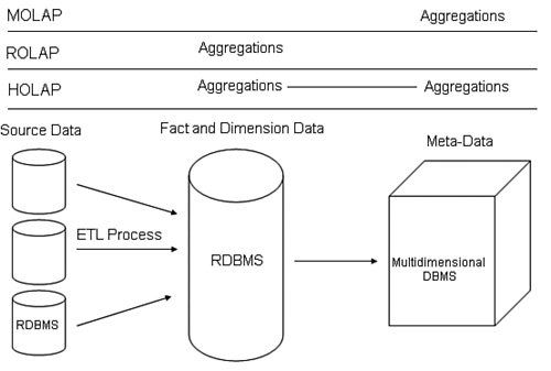
When you click the ellipses next to the aggregations, you are presented with three basic choices for the storage: MOLAP, ROLAP, or HOLAP, as shown in Figure 10-10. These choices have differences in where they store data and how much space the data takes in those locations.

MOLAP stands for multidimensional OLAP, which stores the aggregations in Analysis Services. This is the fastest option but takes the most space to process and during the processing affects the load on the Analysis Services system.

ROLAP stands for relational OLAP, and this option stores the aggregations in the relational system. This has the advantage of lightening the storage and processing load on the Analysis Services system, but at the expense of the relational system. You will often see this arrangement in smaller implementations.

HOLAP stands for hybrid OLAP, meaning that some of the aggregations are stored in the multidimensional system and some in the relational system. This forms a good compromise for both storage and processing.

There are degrees of each of these settings, as displayed in the previous graphic. These nuances have to do with the level of caching the setting provides. The more caching, the more drive space and processing time is needed, but the faster the results for the users when they request them. It is all a tradeoff, with the leftmost setting (ROLAP, low caching) the most beneficial for processing time and space, and the rightmost setting (MOLAP with high caching) the most beneficial for response time.

The diagram in Figure 10-11 shows the entire process and storage options laid out in a single view.

The source data is located on the far left of the diagram in a RDBMS. An ETL process pulls the data through various layers (such as ODS and data marts) to either the data warehouse or some other RDBMS designed to store the facts and dimensions. If you select MOLAP, the aggregations and metadata needed by the OLAP engine are stored in the multidimensional database management system. If you select ROLAP, the aggregations are stored in the RDBMS. If you select HOLAP, it is stored in both.

With those concepts in mind, let's examine how you create and control the storage for the aggregations. Remember, you use the same techniques for the relational data that you have learned throughout this book.

To design an Analysis Services project, you use the Business Intelligence Development Studio. To manage the storage, we will switch back to SQL Server Management Studio.

Instead of choosing a database engine server type of connection on startup, change to an Analysis Services connection, type in the server name as shown in Figure 10-12, and press Enter.

In Figure 10-13, I have expanded all the objects in this screen so that you can see the similarities and differences between this view and the interface in Business Intelligence Development Studio.

Figure 10-13.

[View full size image]

This is the location where the administrator can create or set data sources, create views, and even design cubes. You can do all of those things in the Business Intelligence Development Studio, too, but SQL Server Management Studio also provides access to back up and restore the databases and control security. If you click Connect and select Database Engine as the server type, you can manage all of the levels of the BI landscape from one location, assuming they are in Microsoft SQL Server.

To work with the storage for the Analysis Services system, drill down to the database name you are interested in and then open the Cubes object. Open the cube, and then drill down through the Measure Groups. Open the Facts in the cube, and then open the Partitions object. If the cube has been processed, you will have at least one partition. Right-click the name of any partition, as shown in Figure 10-14.

Figure 10-14.

[View full size image]

From here, you can create a new partition, process the partition, merge it with another, change the aggregation methods, or delete it. To set the storage location for the partition, select Properties from the menu. In the General section shown in Figure 10-15, you can view and set the storage location.

Figure 10-15.

[View full size image]

There is a bit overlap here between what you are able to do in the maintenance phase versus the design phase. It is important that you decide early in the process where you will design and initially create the cube's storage. For the relational parts such as the source system data and the dimensions and facts, you will design, create, and manage the system using SQL Server Management Studio, assuming those objects are stored in SQL Server databases.

For the Analysis Services objects, you can design data sources, data source views, dimensions, measure groups, and partitions in both Business Intelligence Development Studio and SQL Server Management Studio. Significant management tasks such as backing up and restoring are done in SQL Server Management Studio. My recommendation is that you do all design in Business Intelligence Development Studio, including the partition design. The process flows better there. Most management tasks should be accomplished using SQL Server Management Studio, because you have a single place to connect to all the databases in the process.

One of the primary tasks you will be asked to perform is to process the storage after it has been designed and built. I show you how to do that manually using SQL Server Management Studio and automatically using an Integration Services package in a moment. I will explain the various options for processing the partition. This is another area that can be accomplished using Business Intelligence Development Studio; because I consider this a management task, however, I recommend using Management Studio. I have found it cleaner to use Business Intelligence Development Studio for design and SQL Server Management Studio for management and maintenance.

The one exception is in the security area. It is not that you cannot control the security from SQL Server Management Studio, because it is easy to do from there. The consideration for security actually deals more with the way BI is used and controlled. Often in a BI system, the developers are more familiar with the business needs and the rights that groups within the business should have. If the administrator is not part of the design process, it is a two-step task to have them create and control the security. For example, the developer might create a measure that deals with employee salaries. In some cases, a carefully crafted query might be able to show the breakdown of the salaries in the company, so the group that is allowed to see that information must be cleared through the human resources department. The same information can be designed in such a way as to show only an overall figure, and so a wider group is allowed to view it. Unless the administrator is part of that design discussion, the administrator might not be able to assign the rights properly. I explain the security process further in the next section.

Another option you have in dealing with the storage options is to enable a writeback operation on a partition. A writeback operation allows the users of the UDM to alter the data in the fact tables. In fact, the data is not altered at all, but a separate table is created to hold the changes, which the users can view along with the "real" data.

To enable a partition for writeback, drill down to the partition and right-click the Writeback object you see below it. Select Enable Writeback… from the menu that appears. The screen shown in Figure 10-16 will open.

Figure 10-16.

[View full size image]

From here, you can set the table for the altered data and its corresponding data source. After you have created a writeback in a partition, you can disable it if you find it is not being used or you can convert it to a new dimension from the same right-click menu.

Security

The security for Analysis Services is a bit harder to find than the obvious locations in an RDBMS. It is also a bit different in the concepts than in the SQL Server 2005 RDBMS. The reason for this is that the security in Analysis Services is more report based, because a majority of the work in an OLAP system involves queries, not writing data to the database.

In an OLTP system, you focus more on what the users need to do and then build your objects security plan around those needs. When you build objects in Analysis Services, you design the data structures with the most permissive rights in mind. In other words, you design a cube to have everything possibly needed in it. The security in Analysis Services is based on limiting the access from the total cube. Using various methods, you show only the dimensions, facts, and other data to the groups of people that need to see them.

Another difference in Analysis Services security is that it is based entirely on roles. Roles are Windows user or group accounts grouped together based on a security need. There is no platform-based security as there is in the RDBMS, so you do not create any users in the system that are controlled by Analysis Services.

In many ways, using roles based on Windows authentication makes implementing security much simpler. The process involves just three steps: Create the roles, assign Windows users or groups to them, and assign the roles the object permissions.

Let's take a look at an example of creating a role and assigning rights to a cube. This role needs to have the rights to look at any data in a cube called Sales By Time but will not use any writeback operations. This role will also not process or change the project.

As I mentioned earlier, I recommend Business Intelligence Development Studio to handle the security for the project, but you can certainly use SQL Server Management Studio in your implementation, regardless of who handles the security. In this case, I use the Business Intelligence Development Studio.

Open the Business Intelligence Development Studio, and open the project you are interested in. I am using the example project I created in the "Take Away" section at the end of this chapter. To begin, we need to create a role. Once inside the project, open the Solution Explorer, right-click the Roles object, and select New Role. You are immediately placed in a panel that allows you to enter data about the role. The first thing to do is change the name of the role, because it defaults to Role.role. Right-click the name and change it to what you like, but keep the extension of .role. When you do that, you will be asked whether you want to change the object name, too. Although you can have different names for the object than how you refer to it, I recommend you keep them the same unless you have a different need.

When you rename the role, you should enter some descriptive text about what the role is used for. I have entered some information about the Role on this system in Figure 10-17.

Figure 10-17.

[View full size image]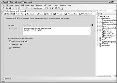

At first glance, it appears that there are only a few options for a role. You can assign it Full Control permission, which means that it has administrative rights to the solution and can make any change or even delete it. You can assign the role the Process database permission, which means it can start a process operation. The only other permission is Read Definition. This permission allows the role to read the structure of the solution. In practice, this is the permission most of the roles will have. We will come to the data part of the permissions in a moment.

The next subtab is Membership, shown in Figure 10-18. This tab controls which Windows accounts are placed in this role.

Figure 10-18.

[View full size image]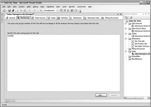

Click the Add button to place any Windows accounts your system has access to in this role.

The next subtab, called Data Sources, sets what this role can see and what rights they have to that source. In this case, I have assigned one data source name and given this role the right to read the data. You can see that tab in Figure 10-19.

Figure 10-19.

[View full size image]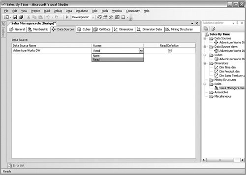

The Cubes subtab shown in Figure 10-20 allows you to set the rights this role has within the cubes. You have a bit more control here because you can allow the role to write data back to the cube or drill through the cube to its source detail. Be careful with this choice because it has performance implications on the network, the Analysis Services system, and even the source system.

Figure 10-20.

[View full size image]

The Cell Data subtab displayed in Figure 10-21 deals with the content of each set of cells within the cube. In this example, I have restricted this role to the count of the Product Class cells. This level of control is powerful and also allows you to set writeback operations or even contingency-based cell access. These are design decisions more than administrative; your developers deal with the way the data is aggregated and displayed long before you get to this screen.

Figure 10-21.

[View full size image]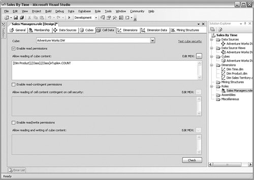

The Dimensions subtab in Figure 10-22 controls which dimensions this role can access and whether they can read them.

Figure 10-22.

[View full size image]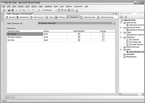

The Dimension Data subtab in Figure 10-23 is similar to the Cell Data subtab. Although it gets a bit confusing for the terminology because of its multidimensional nature, you can think of this subtab as dealing with the horizontal partitioning of the data. Of course, a dimension exists horizontally and vertically, as well as along a Z-axis, but you can extrapolate the idea.

Figure 10-23.

[View full size image]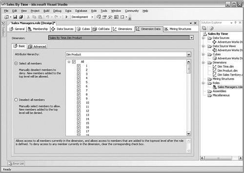

Finally, if you have added data mining structures to your project, you can control the access to them through the Data Mining subtab. You can see that screen in Figure 10-24.

Figure 10-24.

[View full size image]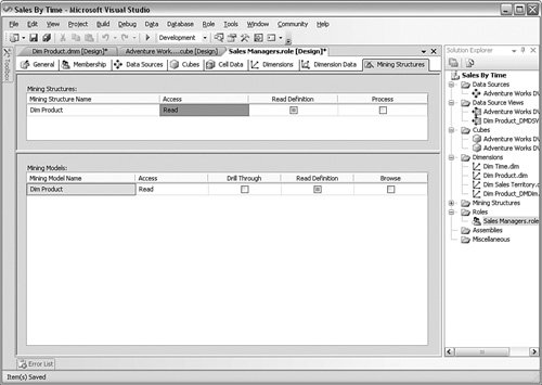

As I mentioned earlier, you can also control and set the security for the model using SQL Server Management Studio. Right-click the Roles object in the database and then select New Role from the menu that appears. You are presented with the same data I just explained in a single set of panels in Figure 10-25.

Figure 10-25.

[View full size image]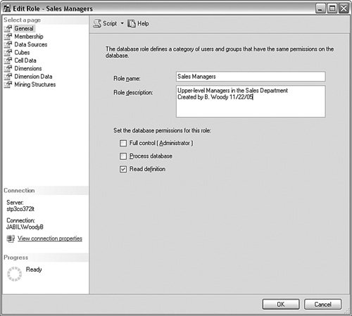

Security for an Analysis Systems project is less about the mechanics, which is quite straightforward, than it is about the design. You will need to work closely with your BI developers if you are asked to manage the security.

Job Processing

After you design and create measure groups, partitions, dimensions, cubes, mining models, mining structures, and databases, you build and deploy them to a production Analysis Services server. In your experimentation thus far you have probably been using the Business Intelligence Development Studio on the server; in production, however, BI developers will use the tool on their own workstations. Before the objects are available on the server to be filled with data, the deployment process creates or updates those objects on the server using a deployment script.

Building the solution creates all the structures and metadata on the local system. Deploying the solution loads those objects to the production server. Deploying the objects is a matter of a few clicks within the Business Intelligence Development Studio. You can see an example of that process in the "Take Away" section at the end of the chapter.

After the project is built and deployed, it needs to be processed. Processing the project involves filling the aggregations with data and creating all the links, metadata, and other database activities in the cube. Until the project is processed, there is no data for the users to see. Even after the data is initially filled in, its source changes over time. To bring the project back to a current data state, you process it again. If the structure of the project or an aggregation calculation is changed, you need to process it again, too.

You do not have to process the entire solution at one time. In most cases, only a few things will change over time, so you can process those as the need arises. You can process at the following levels, from the top down:

• Database

• Cube

• Measure group

• Partition

• Dimension

• Data mining structure

You can process each of those objects, at least to a certain degree. The degree, or processing option, affects how much of the structure and data of each object is processed, which impacts time and computing resources. The more depth you use on the processing, the more recent and complete the data is, but the longer it takes. In many instances, you do not have to reprocess everything, just what has changed.

By a careful selection of what you need to process, how deep you need to process it, and when, you can create an effective level of currency on the system.

It is important to define what level of currency you want for your system. If you ask your users, they will of course want the latest data, all the time. Because of the amount of data a BI system holds, staying current as of the last transaction is not practical. You will need to work with your developers and users to see what part of the system needs from a currency standpoint. Some data needs to be as close to real time as possible, and others can be weeks or even months old. It all depends on what the data is used for.

You can process each object completely or incrementally using SQL Server Management Studio from the Object Explorer, or you can use Business Intelligence Development Studio. You can also run an XML for Analysis (XMLA) script, or you can use AMOs.

Let's take a look at processing the project manually and then examine one of the automated methods. We begin in SQL Server Management Studio. Right-click the object you are interested in and select Process from the menu that appears. The result on my test system is shown in Figure 10-26.

Figure 10-26.

[View full size image]

Select the processing level you want. If you are interested in seeing what will be affected by the processing, click the Impact Analysis button. When you have reviewed that, click OK. You will get a status screen to show you what the system is doing.

Although this is certainly a simple process, you do not want to have to process each object manually. Although you have several choices to automate the process, as I mentioned earlier, one of the most common is to use SSIS. I explained SSIS full in Chapter 8, "Integration Services," so I do not cover the basics again here.

Using Business Intelligence Development Studio, create a new project. Select an Integration Services project template and name it, as shown in Figure 10-27.

Figure 10-27.

[View full size image]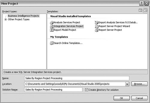

Move to the Control Flow subtab shown in Figure 10-28 and drag an Analysis Services processing item onto the main screen.

Figure 10-28.

[View full size image]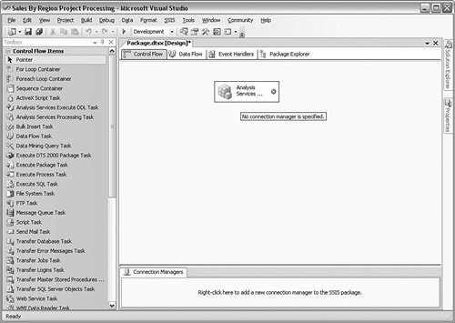

Right-click the bottom part of the screen shown in Figure 10-29 to create a connection to the Analysis server.

Figure 10-29.

[View full size image]

Fill out the screen that comes up with the server name and security information for the package step. When that is complete, double-click the step, and in the General section, enter the screen name and describe it. Click the Analysis Services object in the left part of the panel and set the processing for the objects you want, with the options you are looking for, as shown in Figure 10-30.

Figure 10-30.

[View full size image]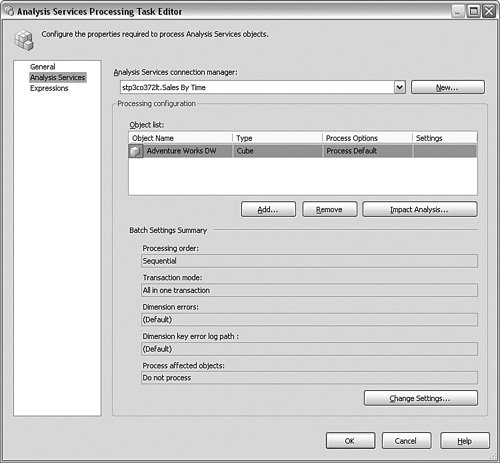

From there, follow the SSIS processes described in Chapter 8 to set up your complete maintenance with alerting, logging, reporting, and the like. You can use scripting or AMO methods in the package if you want a different grain on the process than the Analysis Services Processing object in SSIS. The advantage for using SSIS this way to automate your Analysis Services maintenance is that you can include lots of other logic and actions in one graphical location.

Synchronizing

In a large-scale BI implementation, you often purchase and deploy three sets of systems: development, test, and production. These systems do not always match in size and speed, primarily because of cost. In some cases, you will place the development and testing systems together, but you should never develop or test on a production system.

You will normally purchase and deploy your development landscape first. You will have a few false starts, things you want to do differently, and rapid changes to the system. As the project progresses and shows promise, you will set up your testing system. Normally, you will take greater care in this system to make fewer changes, and do things the "right" way, based on what you have learned in development. When the testing is complete, you are ready to move to production.

In any kind of a sizeable system, it takes a long time to design and deploy the solution. In addition, you will sometimes want to "refresh" your development environment from production so that you have real data to work with. What's needed is a simple way to move an entire project from one place to another. Microsoft calls this process a synchronization and provides a wizard to help you with the process.

To run the wizard, open the SQL Server Management Studio and connect to an Analysis Server. Right-click the Databases object and select Synchronize from the menu that appears. From there, the wizard guides you through selecting the source server and database and imports the database into the server you are on.

The interesting part about this process is that it can happen live. In other words, users can query the database on the destination server while the new one is synchronized. When the synchronization is complete, the new schema is available to the users.

You can also synchronize the system with an XMLA script:

<Command>
 <Synchronize>
 <Source>...</Source>
 <SynchronizeSecurity>...</SynchronizeSecurity>
 <ApplyCompression>...</ApplyCompression>
 <Locations>...</Locations>
 </Synchronize>
</Command>

Backups

Recall that the BI system has different methods of storage for the various layers. The source systems are backed up by the maintenance set up for them independently. For the ODS, data mart, and data warehouse layers as well as the dimensions and facts storage, you still have the same maintenance and recovery scenarios and tools that the OLTP systems have, because they all use a relational database back end. If these are stored in Microsoft SQL Server 2005, you can refer back to Chapter 3, "Maintenance and Automation," for a complete explanation of how to manage those.

The only part of the storage left involves the UDM information, security, and other metadata within the Analysis Services project and the aggregations. These are all stored within the Analysis Services database.

Referring back to the previous graphic showing the aggregation storage in Analysis Services, the location of aggregations is based on which model you chose for the partition's storage (MOLAP, ROLAP, or HOLAP) and the caching options you selected. If you are using MOLAP storage, the backup of the Analysis Services database is larger because the aggregations and potentially the caching are stored there. In the case of HOLAP storage, the backup will be slightly smaller because the aggregations are spread throughout the relational and multidimensional storage engines. With ROLAP storage, the aggregations are placed in the relational storage, so the Analysis Services database backup is much smaller.

Analysis Services database backups are sent to a file, regardless of which storage method you use. You can also restore the Analysis Services database backup to the same server or another or even to another database within any Analysis Services server. Backups are taken at the database level.

In all cases, you can use manual or automated methods for the backups. For the manual method, open SQL Server Management Studio and connect to the Analysis Services server. Right-click the database name you are interested in and select Backup… from the menu that appears. You are presented with a screen similar to Figure 10-31.

Figure 10-31.

[View full size image]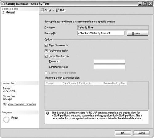

From here, you can set the location for the backup and set compression or security options. You can also back up remote partitions, which are Analysis Services partitions stored on other Analysis Systems servers.

You have several methods available to automate this process, but one of the simplest I have found is to stay within the previous screen and click the Script button on the upper-left side of the screen. That creates an XMLA script of your choices that looks something like this:

<Backup
xmlns="http://schemas.microsoft.com/analysisservices/2003/engine">
 <Object>
 <DatabaseID>Sales By Time</DatabaseID>
 </Object>
 <File>c:\backups\Sales By Time.abf</File>
 <AllowOverwrite>true</AllowOverwrite>
</Backup>

You can copy this script and use it in an AMO or other connection method, but a great way to automate your maintenance is to use a package within Integration Services.

To do that, open the Business Intelligence Development Studio and create a new Integration Services project or use a current one. Create a new task, dragging the Analysis Services Execute DDL item onto the palette. Double-click the item to bring up the screen shown in Figure 10-32.

Figure 10-32.

[View full size image]

On the first panel, set the name of the item. Click the DDL item in the left side of the panel to bring up the panel shown in Figure 10-33.

Figure 10-33.

[View full size image]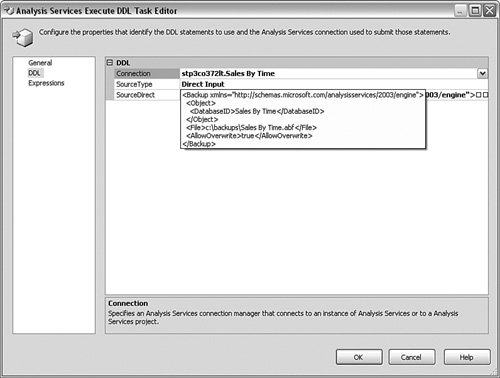

In this panel, choose the connection you want to use (you will need to create one if you do not have one already) and set the SourceType to Direct Input. In the SourceDirect item, click the three dots (ellipses) and paste the code you created in the last step. Save the item and then enter any other maintenance and notification logic you want in the package. By including other items that connect to a relational database, you can create a complete maintenance setup for your entire BI system.

Monitoring and Performance Tuning

Happily, the same monitoring techniques apply as I described in Chapter 5, "Monitoring and Optimization," specifically using Windows System Monitor and SQL Server Profiler. The only difference is that you capture different objects and counters in System Monitor and different trace items in SQL Server Profiler. I do not cover the same ground for the process of collecting here, but let's examine a few of the specifics.

Here are a few of the objects and counters you should collect for Analysis Services.

You should include these counters along with the others I explained in the earlier chapters for overall system health.

For the SQL Server Profiler trace items, the primary objects are those shown here.

You should collect at least the start and stop times for the queries, and if you are interested in specific activity you can capture the text from the items as well as the source connection information and the database name. You can capture several other items to show security, commands, and even notification events. Check Books Online under the topic of "Analysis Services Event Classes" for a full description.