Take Away

In this section, I provide a simple BI solution from end to end so that you can become familiar with the process. Microsoft also includes a similar exercise that you can access from the Windows Start menu in the SQL Server 2005 area. I advise that you start with this example and then go through the Microsoft tutorial. I focus on the entire process and what you have learned in this chapter, and the tutorial focuses more on the tools and mechanics of the process. Using both will help reinforce the concepts and help you get familiar with the tools.

Because we need a common, large database to pull from to adequately demonstrate BI concepts, I will use the AdventureWorks data warehouse example that ships with SQL Server 2005. You will only have the AdventureWorks and AdventureWorksDW databases if you have installed them on your test system. If you would like to follow along with this example and you do not have these databases, just put the installation CD back in the drive and install it on your test system now.

Before you create a BI system, you need a thorough understanding of the business and how it works. I normally do not quote directly from Books Online because you are reading this text for things you do not find there, but in this case I do, because it has the best description of this example company:

Adventure Works Cycles, the fictitious company on which the AdventureWorks sample databases are based, is a large, multinational manufacturing company. The company manufactures and sells metal and composite bicycles to North American, European, and Asian commercial markets. While its base operation is located in Bothell, Washington with 290 employees, several regional sales teams are located throughout their market base.

In 2000, Adventure Works Cycles bought a small manufacturing plant, Importadores Neptuno, located in Mexico. Importadores Neptuno manufactures several critical subcomponents for the Adventure Works Cycles product line. These subcomponents are shipped to the Bothell location for final product assembly. In 2001, Importadores Neptuno became the sole manufacturer and distributor of the touring bicycle product group.

Coming off a successful fiscal year, Adventure Works Cycles is looking to broaden its market share by targeting their sales to their best customers, extending their product availability through an external Web site, and reducing their cost of sales through lower production costs.

This description contains several important BI concepts. For one, it is a large company. That means that our audience for the system will be large, at least for a BI system. A larger audience means people to train on the system, larger and faster hardware, and possibly a heavier load on the networking infrastructure.

Notice also that the company is multinational. That means dealing with multiple currencies, legal definitions, collations, and more.

There are also regional sales teams. That means that there will be a need for granular analysis. Managers at the regions want to know about their site's performance, and managers at headquarters want to know how the entire company is doing.

You can see the questions emerging from a definition of the company and the things managers want to know. From that description, you can begin to develop the formal questions that need to be answered. From those questions, you can investigate the type of data you need to collect, which in turn points you to where you need to get that data. From that information, you can develop a data path, which shows where the data originates (called a source system), where it ends up (called the presentation), and any changes (called transformations) that you do to consolidate and aggregate it. In this chapter, I limit the questions we want to answer to sales of products by time and district.

The AdventureWorks company uses SQL Server 2005 components and features to run their operations and provide a BI landscape. Let's take a look at the source of the data and a little about how it is structured in the data warehouse.

The AdventureWorks database is divided up into several schemas, which have to do with customers, vendors, and employees stored in the People schema, personnel management stored in the HumanResources schema, manufacturing information stored in the Production schema, source vendor information stored in the Purchasing schema, and sales information stored in the Sales schema. These are arranged in typical normalized tables, where unique information is generally stored only once and is referenced to each other through the use of key fields.

The information stored in the AdventureWorks database is used and supported by the company for OLTP applications and reporting. It fills the needs of the first part of the BI system because it provides a source system and a reporting infrastructure.

As the company grew, they needed more analytical mechanisms. Using the SQL Server 2005 database engine, they created a new database called AdventureWorksDW, for their data warehouse. The data in this database is pulled form the OLTP system periodically. One of the decisions you will make when you create your BI system is when and how often you will pull data from the source systems into your reporting subsystem or another storage system for use by Analysis Services.

The data in the AdventureWorksDW database is also structured differently than the OLTP layout. In this database, the data is stored in the dimensions and facts needed for Analysis Services. As you will recall from the spreadsheet example, the columns and rows of the database such as Products and Store Location become dimensions, and the numbers associated with them become the facts. Using the same methodology I showed you earlier in the chapter, the AdventureWorks database forms the source for the star and snowflake schemas found in the AdventureWorksDW database. This database has 16 dimensions, six fact tables, and a few other tables used in KPIs and data mining. In this case, we are going to use a single fact table and a few associated dimensions, just to get familiar with the process.

To begin, open the Business Intelligence Development Studio. Click File and then New and then Project from the menu bar. Leave the project type as Business Intelligence Projects and leave the template selection on Analysis Services Project. Name the project Sales By Time. You can also leave the option set to create a subdirectory for the project.

With that panel filled out as shown in Figure 10-34, click OK to start the process. After the tool creates the directories and sets up the environment, you will be dropped into the project view. On the right side of the tool, you will see a panel called Solution Explorer. It is arranged (conveniently enough) by the steps you take to create the solution. First, you need to connect to a database, arranged by dimensions and facts. In our case, that is the AdventureWorksDW database.

Figure 10-34.

[View full size image]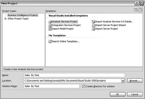

Right-click Data Sources, and then click New Data Source from the menu that appears. You are presented with a wizard (which you can cancel when you are more familiar with the process) that guides you through selecting a database. You can see the process starting in Figure 10-35.

Select Next, and you are placed into the connection definition screen. Because you do not have any connections defined yet, click the New… button on the panel. The next screen has selections for the type of provider (leave it at the default for this exercise), the server and database names, and the security credentials for the connection. Remember, the database you want to connect to is the one that is prepared for use with your Analysis Services system, which in this case is the Adventure-WorksDW database.

Click OK, and you can review the selections that will be used for the connection, shown in Figure 10-36. Click Next to continue. The next panel sets the credentials the solution will use for the project. This might be a different account from the one you used a moment ago. Set this one to Use the credentials of the current user. This means the solution will check what rights the user that is logged on to connect to the source database. Click Next and give the connection a name. In this case, you can leave the defaults. Click Finish to create your connection. You can repeat the process if you need to include sources for more dimensions or facts.

Figure 10-36.

[View full size image]

You now have a connection to the database. Now you need to create either a view of that data or to create a cube. In this case, let's add a simple view of the data. Having a view of exactly what we are looking for simplifies the creation of a cube.

Right-click the Data Source Views object in the Solution Explorer panel on the right. Select New Data Source View from the menu that appears. Once again, a wizard opens to help you through the process. Click Next to continue.

On the Data Source Selection panel, select the Data Source we made in the last step. If this is your first cube it will be the only one. Click Next when you have done that. You are placed in a panel shown in Figure 10-37 where you can select the tables you want to include in this view. Select the dboFactInternetSales and then the arrow icon to move the selection to the right panel.

Figure 10-37.

[View full size image]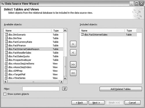

This is where the power of the Intellicube technology really comes into play. Click the Add Related Tables button. After a few moments, the Analysis Services Wizard adds seven tables to the panel, all derived from the relationships and naming in the dimensions and facts.

The wizard adds more than we care about, because we only want to know about sales by product, region, and time. Remove all the tables from the panel on the right, with the exception of the following:

• dbo.FactInternetSales

• dbo.DimProduct

• dbo.DimTime

• dbo.DimSalesTerritory

Figure 10-38 shows what the final selection looks like.

Figure 10-38.

[View full size image]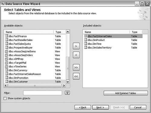

Now click the Next button. Leave the name for the view at the default value. Click the Finish button. The system will process and create the view. You are placed in the graphical representation of the view in a navigation pane, as shown in Figure 10-39.

Figure 10-39.

[View full size image]

Note a couple of interesting things about this view. On the left side of the screen, you can rapidly move through the diagram by clicking the table names. We have a simple diagram in this case, but in more complex uses the diagram can become quite large. In the lower-right corner of the main graphic panel, you can see a small double arrow. Move your cursor over that graphic and click it, holding down the mouse button. This provides a small dynamic view that allows you to quickly move to any section of the diagram. Click any table name or connecting arrow and more information about it shows up in the right side in the Properties panel.

Now right-click the Cubes object in the Solution Explorer and select New Cube from the menu that appears. After the Cube Wizard starts, click the Next button. In the panel shown Figure 10-40, you can have the wizard build the attributes and hierarchies for you, just the attributes, or neither. Notice also that you can build the cube using a template and not a connection to any database, in case it is not available. For this example, leave the defaults.

Click Next to continue, and then select the Data Source View we created a moment ago. Click Next when the wizard completes examination of that data source. In the panel that appears, you are asked to check the boxes next to the facts and dimensions. In this case, the wizard automatically designated them properly. What it did not guess was the time dimension, so select DimTime from the pull-down menu, as shown in Figure 10-41.

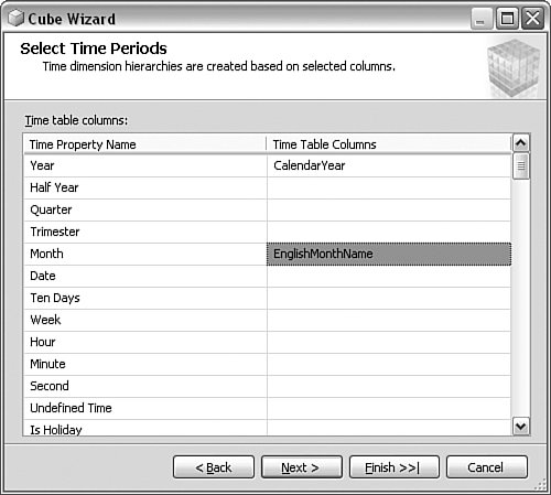
After you have set the time dimension, click Next to continue. Because we defined a time dimension that has multiple attributes, the wizard wants to know how we will break them into levels. In our case, we are interested in years and months. The source table contains many more breakdowns than that, so this panel allows us to assign which fields provide the levels we want. In this case, select Year to map to the CalendarYear field, and Month to map to the EnglishMonthName field, as shown in Figure 10-42.

In the next panel, you can set the measures (facts) that you want to include in the cube. In many cases, you will store lots of facts in a single fact table, especially when they occur in the same time period. To keep this example simple, we want only the FactInternetSales item, all the keys, and the SalesAmount facts. De-select everything except those items, as shown in Figure 10-43.

Figure 10-43.

[View full size image]

Click the Next button. The wizard will detect any hierarchies in the data. When that is complete, you can review the layout before it is finalized. Click the Next button, leave the name of the cube at the defaults, and click the Finish button. The system creates the cube and drops you into the graphical panel displayed in Figure 10-44, which is similar to the data source view you worked with earlier.

Figure 10-44.

[View full size image]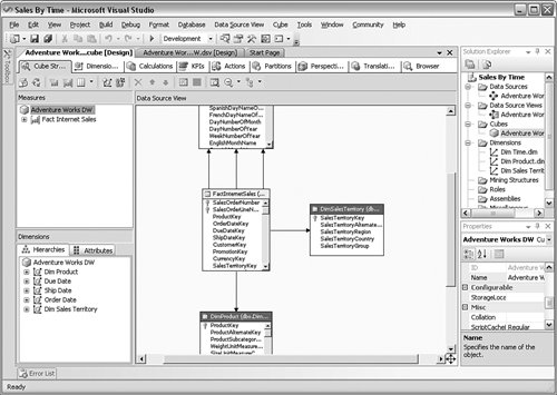

Although this graphical view works the same way as the data source view graphic, you have different items to work with in the main panel; and if you look at this busy screen closely, you will notice several subtabs within the main tab. These views show the dimensions, allow you to work with calculated members, create perspectives, and more. To keep this example simple, let's process the cube as it is and then take a look at the results.

At the moment, the cube is defined and designed. However, there is no OLAP database for the project, and so there is no data to display. To create the database, we need to deploy it. Before we do that, we need to design the storage the database uses. As explained earlier in this chapter, you need to make a tradeoff between storage size and the responsiveness of the system. The more responsive the system is, the more aggregations it uses. The more aggregations it uses, the more space it takes.

In this case, click the subtab marked Partitions. Next to the Molap 0% item, click once on the button that has three dots on it, as shown in Figure 10-45.

Figure 10-45.

[View full size image]

When you click that button, another wizard appears. Click Next and leave the slider selection at the MOLAP selection, as shown in Figure 10-46.

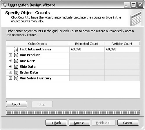
Click Next to continue. Click the Count button on the next panel to have the wizard automatically figure out how many calculations it needs to make (see Figure 10-47).

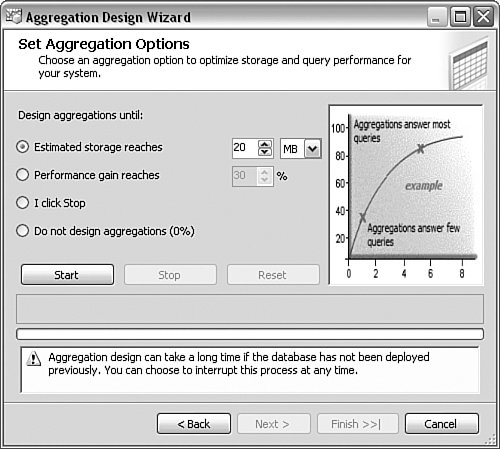
On the panel shown in Figure 10-48, you can limit how much space or time you want the wizard to spend calculating the aggregations. If your test system is short on space, enter a number you can live with for the space; otherwise, pick a percentage gain you want to use for optimizing the aggregations. The higher the numbers you place here, the higher the performance.

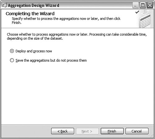
Click the Next button and allow the wizard to complete. When it finishes, it will display the amount of space it will use and the number of aggregations it created, as shown in Figure 10-49. Click Next. Change the selection on the next panel to Deploy and process now, and then click the Finish button.

The system will pause for a moment or two and then present you with a Run selection. The options here determine how much of an impact to the system the process will take. In this example, leave the Process Full option set and click the Run button. The system will then create the aggregations. When that process completes, you can close the processing panel.

Now we can view the fruits of our labor. Click the Browser subtab in the Business Intelligence Development Studio tool, in the Adventure-Works cube. It is the last subview in the screen. Open the measures you see and drag any fact into the center part of the panel on the right. Now expand a dimension and drag an item from into the thin bars across the top and sides of the section on the right, as shown in Figure 10-50.

Figure 10-50.

[View full size image]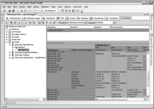

In this example, I have placed the Sales Amount fact from the Fact-InternetSales measure in the center area. I have also added the Model Name dimension from the Dim Product dimension in the far-left side of the vertical bar. After that, I added the Sales Territory Region from the Dim Sales Territory dimension next to that same bar. Along the top horizontal bar, I added the Calendar Year dimension from the Ship Date dimension.

This quickly shows me the sales for the various regions for all the products I am interested in, by month. Even with this simple example, I can quickly change the view to see the due dates and sales by month, use other languages (they were included in the source start schema), and more.

You can certainly do more with this example. Take some time and add a data mining exercise to this cube to see whether you can determine any patterns in the data and to what level of certainty they show. You can also add KPIs to this project to show any deviations from the norms you establish within the solution.

If you are interested in reviewing a real-world example of using a SQL Server 2005 implementation for large-scale BI, search inside Microsoft's TechNet site for "Project REAL." It is a complete set of white papers detailing that effort.