Changing Worksheet Views
One of Excel's greatest strengths is its flexibility. You can change the look of the Excel screen to match the work you're doing. For example, if you've opened several workbooks, you can set your screen so that all of them are visible. If you're working on a complicated project, you can maximize the program and adjust the screen view to magnify your data. Other times you can zoom out to see more of the worksheet. You can even split a large worksheet into separate windows, called panes, to keep you from scrolling back and forth.
Arranging Open Workbooks
If you're working with more than one Excel workbook, jumping back and forth between them becomes tedious very quickly. Instead of viewing one file at a time, you can set Excel to display all the open files on the screen.
To Do: Arrange Open Workbooks
When you've opened more than one Excel workbook, click the Window menu and choose Arrange. The Arrange Windows dialog box, shown in Figure 4.8, appears.
Figure 4.8. The Arrange Windows dialog box enables you to set your screen to view more than one workbook.
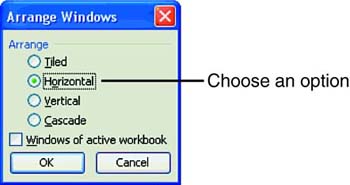
Click the option button next to the option you want. The following options are available:
Tiled? The open workbooks are arranged in individual tiles; the more open files, the smaller the individual tiles.
Horizontal? The workbooks are displayed in horizontal strips.
Vertical? The workbooks appear in vertical strips.
Cascade? The workbooks are reduced in size and displayed diagonally. The top workbook is the active one. If you chose this option, you'll need to click in one of the inactive workbooks to bring it to the top.
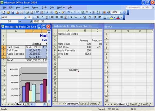
Click OK to close the Arrange Windows dialog box. The workbooks are arranged on your screen in the view you selected. Figure 4.9 shows a vertical arrangement of three windows.
Figure 4.9. Arrange windows in vertical strips.
Each time you open a workbook file, an icon for that file appears on the Windows taskbar. Position your mouse pointer in the taskbar icon to see the full name of the file. Even if you don't arrange the workbooks on your computer screen, you can easily see how many workbook files are open by looking at the taskbar. |
Comparing Workbooks Side by Side
Comparing data in two open workbooks and bouncing from one to the other to view the data can be a painstaking task. Instead of examining one file at a time, you can set Excel to display both open files side by side on the screen.
With the two workbooks open, choose Window, Compare Side by Side. Excel displays one workbook in the top half and the other in the bottom half of the Excel window. You also see the Compare Side by Side toolbar, as illustrated in Figure 4.10.
Figure 4.10. Compare Side by Side lets you compare data in two workbooks at once.
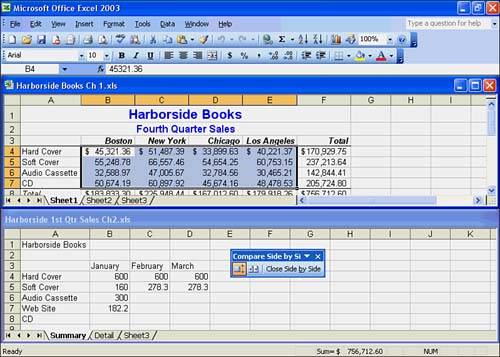
You can scroll simultaneously in both workbooks, but if you want to turn off this feature, click the Synchronous Scrolling button on the Compare Side by Side toolbar. If you want to reset the window position in a workbook, move to the new location in one of the workbooks, and click the Resets Window Position button on the Compare Side by Side toolbar. To return to viewing individual workbooks, click the Break Side by Side button on the Compare Side by Side toolbar.
Zooming In and Out
Change the view of your worksheet by zooming in and out. To change the zoom percentage, click the Zoom button on the Standard toolbar. Choose the size at which you want to view the screen.
The lower the percentage, the more you see of the screen. However, at a low percentage, like 25%, you probably won't be able to read the text. Use the low percentages to examine the look of the screen. If you choose a high percentage, you see less of the total screen, but each cell appears larger.
Another way to adjust the change the zoom percentage is to click the View menu and choose Zoom. The Zoom dialog box, as shown in Figure 4.11, enables you to choose from a variety of magnification levels. The Custom selection allows you to specify a level as low as 10% or as high as 400%.
Figure 4.11. The Zoom dialog box lets you control the view of the screen.
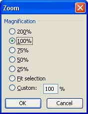
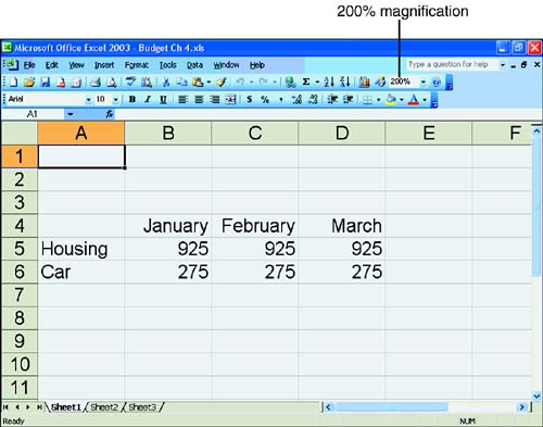
Figure 4.12 shows data on a worksheet at a magnification level of 200%.
Figure 4.12. Zooming in to get a closer look at your data.
Additionally, you can highlight a block of cells and choose Fit Selection to magnify the block so that its cells all fit in the window. After you adjust the Zoom magnification, you can change it back or switch to a new percentage at any time.
Changing to Full-Screen View
Most times, when you're working in Excel, it's helpful to be able to see the toolbar buttons, the title bar, and other screen elements. However, these elements take up valuable screen real estate and reduce your viewing area. Excel makes it easy to switch to a full-screen view, in which the worksheet, sheet tabs, and menu bar are displayed. You can toggle between full-screen and normal view at any time.
To display the worksheet in full-screen view, click the View menu and choose Full Screen. Your screen should look similar to the one in Figure 4.13.
Figure 4.13. Full-screen view shows more of the worksheet.
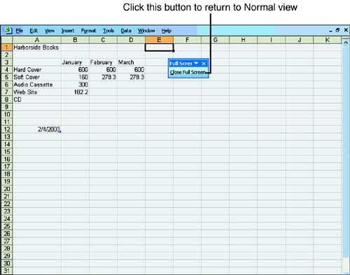
If you absolutely need to work with a toolbar in full-screen view, open the View menu and click the toolbar you want to display. (Displaying more than one toolbar defeats the purpose of switching to full-screen, so add toolbars sparingly.) To return to normal view, click the Close Full Screen button.
Keeping Row and Column Headings Visible
Many large worksheets contain row and column headings that identify the data. However, as you scroll the worksheet, the headings become obscured. Instead of trying to guess which row or column heading matches the current cell, you can freeze the headings into panes. Here's how:
Freeze the top horizontal pane by clicking the row below where you want the split to appear.
Freeze the left vertical pane by clicking the column to the right of where you want the split to appear.
Freeze both the upper and left panes by clicking the cell below and to the right of where you want the split to appear.
Pane?
![]() An individual section of a window.
An individual section of a window.
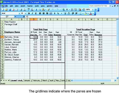
Next, click the Window menu and choose Freeze Panes. Figure 4.14 displays a worksheet window that has been split into panes. The row and column headings remain on the screen as you scroll through the worksheet, enabling you to always know where you are. You can unfreeze the window any time by clicking Window, Unfreeze Panes.
Figure 4.14. The row and column headings remain constant.