Formatting with AutoFormat
Excel's AutoFormat feature takes away some of the hard work involved in formatting a worksheet. AutoFormat provides you with 16 predesigned table formats that you can apply to a selected range of cells on a worksheet.
Instead of applying each format to your data, one at a time, you can apply a group of formats in one shot with one of Excel's predesigned formats. The AutoFormat command lets you select a format and transform your table with a couple of mouse clicks.
In this To Do exercise, you get to try out a predesigned format using the AutoFormat command.
To Do: Apply an AutoFormat
Select the cells that contain the data you want to format; in this case, select cells A3:D9.
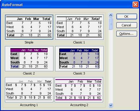
Choose Format, AutoFormat. The AutoFormat dialog box pops open, as shown in Figure 10.10. You see a palette of predesigned table format samples, each with a name.
Figure 10.10. Predesigned table formats in the AutoFormat dialog box.
Scroll through the table format samples. Stop at the List 2 sample.
Click the List 2 sample table format.

To view the elements that make up the selected table format, click the Options button. You can turn off any Format option to customize the look of the table format.
Click OK. Excel formats your table to make it look like the one in the sample you selected. It looks great!
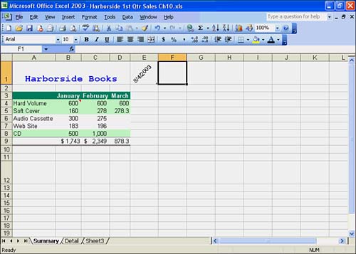
Click any cell to deselect the range. Figure 10.11 shows the table formatted with the List 2 AutoFormat. The green bars make the worksheet more attractive and readable.
Figure 10.11. The worksheet formatted with the List 2 AutoFormat.
What if you don't like what AutoFormat did to your worksheet? No problem. To remove a prefab format, press Ctrl+Z to undo the format. |


