Modifying a Pivot Table

After you build a pivot table, you can make changes to it any time. For example, if you want to examine the new clients for a particular month, you need to change the Month field. Use the drop-down list to the right of the field name. Select a month and click OK. This step selects and deselects new clients in the list, and Excel instantly displays new clients broken down by more or less magazines in the DATA area of the pivot table. You also should see the grand total dollar amounts by magazine at the bottom of each item. At the bottom of the table, you should see the grand total for new clients to all magazines.

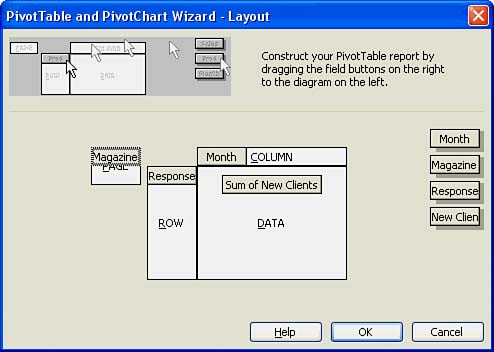
You can use this report to analyze your data in various ways. For instance, click the PivotTable down arrow button on the PivotTable toolbar, choose PivotTable Wizard, and click the Layout button. Drag the buttons off the diagram, and arrange the fields like this: Magazine in the PAGE area, Month in the COLUMN area, New Clients in the DATA area, and Responses in the ROW area. The completed PivotTable dialog box should look like the one in Figure 18.7.

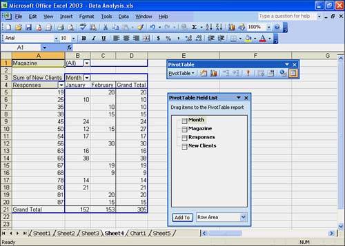
The pivot table now illustrates sales by cost for each item. All items are selected in the column field, and you should see the total item quantity for all the items. You can use the Cost row field to restrict cost shown to each individual item. Figure 18.8 shows the pivot table derived from rearranging the data.

The PivotTable toolbar provides tools for working with pivot tables. Table 18.1 lists those tools and what they can do for you.

Below the buttons on the PivotTable toolbar, you should see the PivotTable Field List window. The field buttons that you dragged to the PAGE, ROW, COLUMN, and DATA areas in the PivotTable diagram appear in the window. You can drag a field button from the window to the PivotTable at any time to rearrange the data in your pivot table.

Some other changes you might want to make to your pivot table include removing and adding fields in the pivot table. To remove fields, drag the field item buttons off the PivotTable. Excel indicates in the pivot table exactly where you should place a field button. For example, in the PAGE area, you should see "Drop the page field here." To add fields to the pivot table, drag the fields from the PivotTable Field List window into the PAGE, COLUMN, ROW, and DATA areas marked on the PivotTable. By using the PivotTable Field List window, you can build new or different pivot tables in a snap.

You can change the computation for the numbers. By default, the numbers are added with the SUM function, but you can change to AVERAGE, MIN, or MAX. For example, if you want to average the numbers instead of summing them, double-click the Sum of New Clients button in the DATA area. The PivotTable Field dialog box opens, as shown in Figure 18.9.

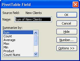
Choose Average and click OK. Excel changes the Sum of New Clients to Average of New Clients.

To change the format of numbers in a PivotTable, open the PivotTable Field dialog box, click the Number button and choose a number format. Click OK.

If you want to group PivotTable items and create a new field for the items as a group, select the cells you want to group. Choose Data, Group and Outline, Group. Excel creates a new field that contains the selected items.

To group items automatically, select one item in a field. Choose Data, Group and Outline, Group. In the Group Dialog box, in the By list, select the grouping options you want. Then click OK. Excel creates the groups based on the options you selected.